Sometimes you read an academic article and the author fills in the data gaps with interpolation. That is, they assume some functional form of the data and then replace the missing values with the estimated ones. Often, lacking an informed opinion about functional form, authors will just linearly interpolate between the closest known values. Sometimes this method is OK. But sometimes we can do better.
Historical census data provides a good example because the frequency was only every ten years. Say that we want to know more about child migration patterns between 1850 and 1860. What happened in the intervening years? Who knows. Let’s look at the data.
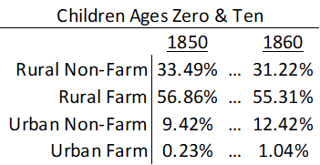
Using data on individuals who have been linked across censuses allows us to fill in the gaps a little bit. For simplicity, let’s just look at whether a child migrant lived in an urban location and whether they lived on a farm. That means that there are 4 possible ways to describe their residence. Below is a summary of where children migrants lived at the age of zero in 1850 and where the same children lived a decade later at the age of ten in 1860 given that they moved counties.
When I’m the mean time did these children move from one place and to the other? We don’t know exactly. The popular answer is to say that they moved uniformly throughout the decade. That’s ‘fine’. But it assumes that the rate at which people departed places was rising and the rate at which they arrived places was falling. Maybe that’s true, but we don’t really know. Below-left is a graph that shows the linear interpolation.

The nice thing about linear interpolation is that everyone is accounted for at each point in time. The total number of people don’t rise or fall in the intervening interpolation period. But if we were to assume that children departed/arrived at each type of place at a constant rate (maybe a more reasonable assumption), then suddenly we lose track of people. That is, the sum of people dips below 100% as people depart faster than they arrive.
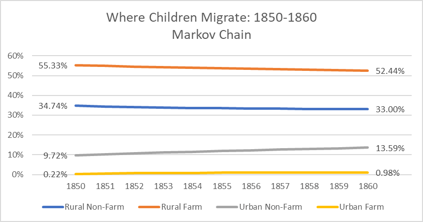
What’s the alternative to linear interpolation?
The alternative method is to use a transition matrix. A transition matrix allows us to be more refined about where people live. If children in 1850 leave one place and arrive at another, then the 1851 population distribution should reflect this. The complexity is that people can leave one type of household and move to any of the household types – including the original. Given that we know the beginning and ending child migrant populations for individuals, we can build a richer picture of where people start and where they end up. Below is a matrix that describes just that.
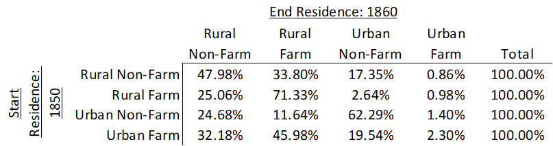
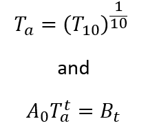
How does this help? The above describes how children moved or transitioned between 1850 and 1860. If ‘A0’ describes the 1850 population, matrix B10 describes where they lived in 1860, and T10 is the above matrix, then we have just found:

Since T is the decadal transition matrix, we can essentially take the 1/10th power in order to find the annual transition matrix (Some math happens here that I am glossing over). Such that:
We can vary the exponent on Ta in order to find the average migrant residence distribution in the years between the known beginning and end distributions. The results below provide us the nice gradual rates that geometric interpolation provides while also keeping track of everyone. The fancy name for this process is a Markov chain. But more people know what you’re talking about if you just say transition matrix.