Economist Writing Every Day

Excel is an attractive tool for those who consider themselves ‘not a math person’.  In particular, it visually organizes information and has many built-in functions that can make your life easier. You can use math if you want, but there are functions that can help even the non-math folks

If you are a moderate Excel user, then you likely already know about the AVERAGE and COUNT functions. If you’re a little but statistically inclined, then you might also know about the STDEV.S function (STDEV is deprecated). All of these functions are super easy and only have one argument. You just enter the cells (array) that you want to describe, and you’re done. Below is an example with the ‘code’ for convenience.

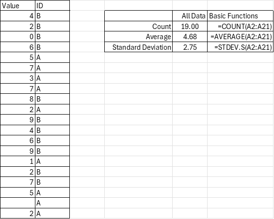
=COUNT(A2:A21)
=AVERAGE(A2:A21)
=STDEV.S(A2:A21)

If you do some slightly more sophisticated data analysis, then you may know about the “IF” function. It’s relatively simple; if a proposition is true (such as a cell value condition), then it returns a value. If the proposition is false, then it returns another value. You can even create nested “IF”s in which a condition being satisfied results in another tested proposition. Back when excel had more limited functions, we had to think creatively because there was a limit to the number of nested “IF” functions that were permitted in a single cell. Prior to 2007, a maximum of seven “IF” functions were permitted. Now the maximum is 64 nested “IF”s. If you’re using that many “IF”s, then you might have bigger problems than the “IF” limitations.

Another improvement that Excel introduced in 2019 was easier array arguments. In prior versions of Excel, there was some mild complication in how array functions must be entered (curly brackets: {}). But now, Excel is usually smart enough to handle the arrays without special instructions.  Subsequently, Excel has introduced functions that combine the array features with the “IF” functions to save people keystrokes and brainpower.

Looking at the example data we see that there is an identifier that marks the values as “A” or “B”. Say that you want to describe these subgroups. Historically, if you weren’t already a sophisticated user, then you’d need to sort the data and then calculate the functions for each subgroup’s array. That’s no big deal for small sets of data and two possible ID values, but it’s a more time-consuming task for many possible ID values and multiple ID categories.

The early “IF” statements allowed users to analyze certain values of the data, such as those that were greater than, less than, or equal to a particular value. But, what if you want to describe the data according to criteria in another column (such as ID)? That’s where Excel has some more sophisticated functions for convenience. However, as a general matter of user interface, it will be clear why these are somewhat… awkward.

COUNTIFS

The syntax of “COUNTIFS” let’s you list arrays with identical dimensions and corresponding criteria. The general syntax requires a one-two punch: “condition array, criteria, condition array, criteria, condition array, criteria”… The criteria are all combined with an unwritten “AND” function. That is, all of the criteria must be met in order to count an item. In the particular code below, I count the number of values with an ‘A’ ID that are not blanks.

=COUNTIFS(A2:A21,"<>",B2:B21,"A")
=AVERAGEIFS(A2:A21,B2:B21,"A")
=AVERAGEIF(B2:B21,"A",A2:A21)

AVERAGEIFS

The “AVERAGEIFS” function is similar. It calculates the average of a subsample that meets some criteria. Conveniently, the criteria can be on any array with identical dimensions including the values themselves. The syntax is very similar to that of COUNTIFS. Here, it’s “value array, condition array, criteria, condition array, criteria”… Inconveniently, this syntax is different from AVERAGEIF without the “S”. The AVERAGEIF function places the value array in the last argument. Why? Who knows! It’s probably a difference due to legacy.

STDEV.S & IF

The problem with the specialized functions that combine COUNT or AVERAGE with IF is that it essentially doubles the number of possible Excel functions – and triples the number of functions if we also include IFS. In some sense, every single function should have additional versions that include an IF or IFS. But that’s not the world in which we live. We have a few functions supplemented with built-in IFs for convenience, but the user must figure it out on their own otherwise.

The STDEV.S function is such a function. IF statements don’t always work despite advice that you can find online. Rather, a robust and generalizable method is to use the FILTER function (not to be confused with proper-case Filter, which changes the list-order of the data). The syntax is “value array, array condition statement, [empty set result]”. That last argument is an optional value that you want returned if the filter results in an empty set. What makes the FILTER function especially valuable is that you don’t need to memorize which commands have built-in versions with an IF or IFS suffix. You can always use filter on any function that expects an array.  The example below replicates all of the IFS functions by using the basic version of the commands and supplementing with the FILTER function.

=COUNT(FILTER(A2:A21,B2:B21="A"))
=AVERAGE(FILTER(A2:A21,B2:B21="A"))
=STDEV.S(FILTER(A2:A21,B2:B21="A"))

In summary, you can add FILTER to most functions to build your own conditional functions. The syntax will always be the same, unlike AVERAGEIF and AVERAGEIFS, and you don’t need to memorize or hope that Excel made an accommodation for you. Just use the FILTER function and live your life freely on your own terms, without needing accommodation from anyone.