Economist Writing Every Day

I just learned about the Bayesian Dawid-Skene method. This is a summary.

Some things are confidently measurable. Other things are harder to perceive or interpret. An expert researcher might think that they know an answer. But there are two big challenges: 1) The researcher is human and can err & 2) the researcher is finite with limited time and resources. Even artificial intelligence has imperfect perception and reason. What do we do?

A perfectly sensible answer is to ask someone else what they think. They might make a mistake too. But if their answer is formed independently, then we can hopefully get closer to the truth with enough iterations. Of course, nothing is perfectly independent. We all share the same globe, and often the same culture or language. So, we might end up with biased answer. We can try to correct for bias once we have an answer, so accepting the bias in the first place is a good place to start.  

The Bayesian Dawid-Skene (henceforth DS) method helps to aggregate opinions and find the truth of a matter given very weak assumptions ex ante. Here I’ll provide an example of how the method works.

Let’s start with a very simple question, one that requires very little thought and logic. It may require some context and social awareness, but that’s hard to avoid. Say that we have a list of n=100 images. Each image has one of two words written on it, “pass” and “fail”. If typed, then there is little room for ambiguity. Typed language is relatively clear even when the image is substantially corrupted. But these words are written, maybe with a variety of pens, by a variety of hands, and were stored under a variety of conditions. Therefore, we might be a little less trusting of what a computer would spit out by using optical character recognition (OCR). Given our own potential for errors and limited time, we might lean on some other people to help interpret the scripts.

The setup is straight forward. All we want to know is whether each image says “pass” or “fail”. We will use something akin to the wisdom of crowds, but with a bit more thought than simple democracy or averages. Let’s code “pass”=1 and “fail”=0. If we have 6 users evaluating the images, then the first portion of our data might look like the below. We could just calculate the average for each image, but that has shortcomings. Specifically, it ignores any priors about the number of 1’s and it ignores whether the users make mistakes in unique ways.

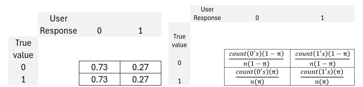
Let’s address the first issue. The DS method adopts a prior of a 50-50 split between 1’s & 0’s absent other information. It turns out that this prior doesn’t matter much. The further the prior is from the truth simply increases how much information we need in order to solve our problem. For our current example, let’s adopt a prior that there are 20 of the 100 images including the word “pass”, or π =20%. Given the difficulty of the problem, it stands to reason that incorrect designations are possible. As a starting point, we can expect that a user will answer with a 1 for 20% of responses. Therefore, without any bias in how a user makes mistakes, we would expect the below matrix. Notice that the possible user responses sum to 1 under each true value. This is called a confusion matrix and it describes a user’s correct and incorrect designations. It’s a 2×2 matrix because it includes two possible responses and two possible true states of the world.

The above makes a strong assumption of unbiased symmetry in how a person makes mistakes. Real people have their own biases, however. Let’s say that user_1 answers with 27 1’s and 73 0’s. That results in the confusion matrix below followed by the math. Some things in the math look redundant, but I’ll address it later. Each person has their own unique confusion matrix.

Once we have a confusion matrix for each person, we can calculate the likelihood of seeing the actual user responses under the assumption that the true label is 1 for an individual image. We can do the same assuming that the true label is 0.

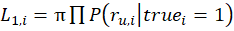
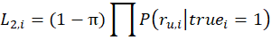
Now we can say: given what the user answers are, what is the probability that the true state of an image is 1, or “pass”. That is simply:

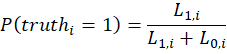
Skipping a whole bunch of math, you would find that the unsatisfying result that all images have a 20% posterior probability of being true. This occurs because our likelihoods are proportional to one another, cancelling each other our and resulting in the posterior that’s identical to the prior of π=0.2. The solution is to A) identify a unique prior for every image or B) introduce a smoothing parameter. If we could do A), then we probably wouldn’t be doing any of this, or maybe we would just be auditing an OCR model. Given that we adopt a low-hubris position of not asserting the ex ante state of any image, we’ll opt for a smoothing parameter, α. The smoothing parameter enters the confusion matrix equation as reflected below.

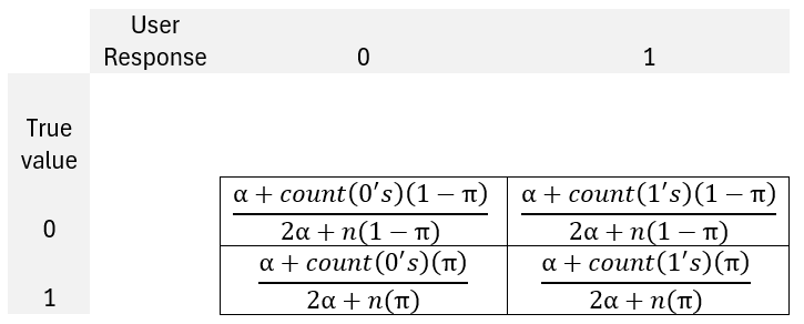
What does the smoothing parameter achieve? It causes the confusion matrix values to diverge from the priors in a way that is unique to each person. The smoothing operator creates some heterogeneity among the estimated probability that each image is 1 because that probability is dependent on the likelihoods stats, which are in turn dependent on the confusion matrices.

All of this is kinda blah – Until now. The now heterogeneous posterior probabilities for each image can be fed back into the confusion matrix. The new matrix is reflected below. The 1[…] notation is an indicator function and, for the sake of space, the W refers to the sum of the numerators within each True value. Of course, this feeds back into the likelihood stats, and yields new posterior probabilities for each image. The beauty is that people who are smarter than me have shown that this process is convergent. That is, we’ll get a distribution of posterior image probabilities for each smoothing parameter.

But what exactly is the smoothing parameter? It’s just a non-negative constant. Using a value of 1 is the classic default. A smaller value causes faster convergence, but also may cause the confusion matrices to change a lot with each iteration. A larger smoothing parameter is more conservative, and requires more iterations or more data. Regardless of the possible concerns, the practical applications of the Bayesian Dawid Skene method can do great things, often with just a few users and a few iterations of the algorithm.

Some advantages of the method include:

• Adjustments for difficult to interpret images
• Permits missing data
• Differentiates user designation error types

Here is a cool paper that discusses the performance of the method more (spoiler alert, it’s the best):

Paun, Silviu, Bob Carpenter, Jon Chamberlain, Dirk Hovy, Udo Kruschwitz, and Massimo Poesio. 2018. “Comparing Bayesian Models of Annotation.” Transactions of the Association for Computational Linguistics 6 (December):571–85. https://doi.org/10.1162/tacl_a_00040.