Economist Writing Every Day

All of us have assets. Together, they experience some average rate of return and the value of our assets changes over time. Maybe you have an idea of what assets you want to hold. But how much of your portfolio should be composed of each? As a matter of finance, we know that not only do the asset returns and volatilities differ, but that diversification can allow us to choose from a menu of risk & reward combinations. This post exemplifies the point.

1) Describe the Assets

I analyze 3 stocks from August 1, 2024 through August 1, 2025: SCHG (Schwab Growth ETF), XLU (Utility ETF), and BRK.B (Berkshire Hathaway). Over this period, each asset has an average return, a variance, and  co-variances of daily returns. The returns can be listed in their own matrix. The covariances are in a matrix with the variances on the diagonal.

The return of the portfolio that is composed of these three stocks is merely the weighted average of the returns. In particular, each return is weighted by the proportion of value that it initially composes in the portfolio. Since daily returns are somewhat correlated, the variance of the daily portfolio returns is not merely equal to the average weighted variances. Stock prices sometimes increase and decrease together, rather than independently.

Since the covariance matrix of returns and the covariance matrix are given, it’s just our job to determine the optimal weights. What does “optimal” mean? This is where financiers fall back onto the language of risk appetite. That’s hard to express in a vacuum. It’s easier, however, if we have a menu of options. Humans are pretty bad at identifying objective details about things. But we are really good at identifying differences between things. So, if we can create a menu of risk-reward combinations, then we’re better able to see how much a bit of reward costs us.

2) Create the Menu

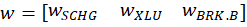
In our simple example of three assets, we have three weights to determine. The weights must sum to one and we’ll limit ourselves to 1% increments. It turns out that this is a finite list. If our portfolio includes 0% SCHG, then the remaining two weights sum to 100%. There are 101 possible pairs that achieve that: (0%, 100%), (1%,99%), (2%,98%), etc. Then, we can increase the weight on SCHG to 1% for which there are 100 possible pairs of the remaining weights: (0%,99%), (1%, 98%), (2%, 97%), etc. We can iterate this process until the SCHG weight reaches 100%. The total number of weight combinations is 5,151. That means that there are 5,151 different possible portfolio returns and variances. The below figure plots each resulting variance-return pair in red.

Each portfolio that is entirely composed of one stock is noted in black. The highest possible return would have been achieved by holding 100% SCHG. But, the variance minimizing portfolio, noted in green, includes some of all three assets (the weights are also displayed). That is, even though BRK.B had the lowest return and middling volatility, it still plays a part in the most stable portfolio. The same variance-minimizing portfolio would have been unachievable without BRK.B.

However, the goal isn’t always to minimize variance. We’d like to maximize the return at any variance that we adopt. The blue line is the ‘Efficient Frontier’ which denotes exactly that. The blue line is the menu of portfolios, differing by asset weight, that tell us the trade-off among the return maximizing variances (or the variance minimizing returns). Note that the blue line doesn’t border the lower portion of the possible portfolios, where the slope would be negative. This is because higher returns would be possible at each corresponding level of portfolio variance.

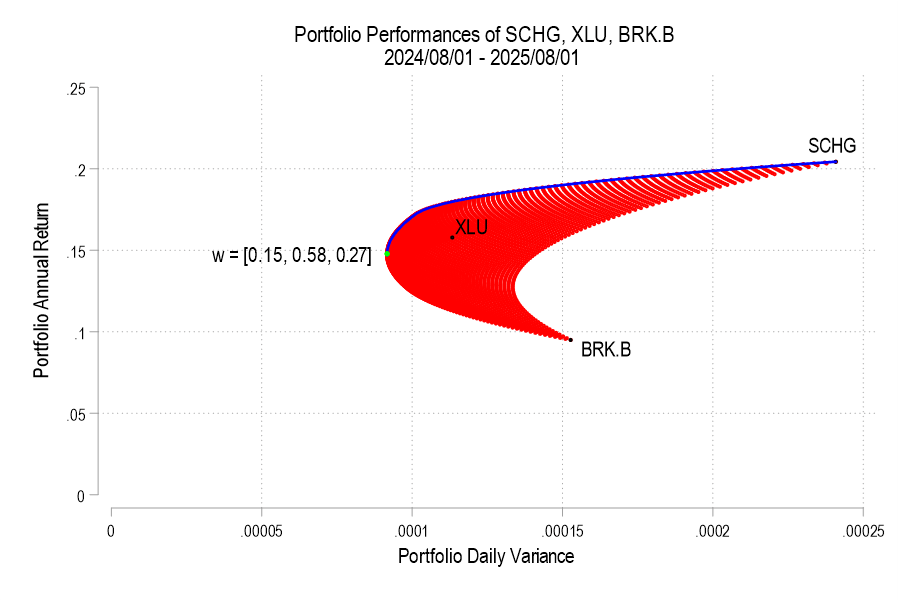
Another important insight is that adding another possible asset to the set of portfolios never reduces your options. For example, if I mistakenly omitted BRK.B from the possible set of assets because it has the lowest return, and instead only included SCHG and XLU, then I’d not improve my menu of efficient allocations. In fact, in this case, I would yield only a subset of my previous menu of return-variance combinations. The below figure shows the 2-asset efficient frontier in red and the 3-asset efficient frontier in blue.

3) Choose from the Menu

In the case above, there were 5,151 possible portfolios, each differentiated by their asset weights. That’s a daunting set of options. So, the efficient frontier narrows the options to those which provide the highest portfolio return at each portfolio variance. This is where you can see your trade-offs. If you are at the variance minimizing weights, then adopting a little bit of volatility provides a lot of additional reward. But, if you adopt the return maximizing weights, then you can reduce your volatility substantially without giving up much return. This is kind of like the Production Possibility Frontier (PPF) in economic theory. Except, instead of a marginal rate of transformation (MRT) that trades-off between different outputs, the above menus tradeoff among the different risks and rewards.