Are Your Portfolio Weights Right?

What do portfolio managers even get paid for? The claim that they don’t beat the market is usually qualified by “once you deduct the cost of management fees”. So, managers are doing something and you pay them for it. One thing that a manager does is determine the value-weights of the assets in your portfolio. They’re deciding whether you should carry a bit more or less exposure to this or that. This post doesn’t help you predict the future. But it does help you to evaluate your portfolio’s past performance (whether due to your decisions or the portfolio manager).

Imagine that you had access to all of the same assets in your portfolio, but that you had changed your value-weights or exposures differently. Maybe you killed it in the market – but what was the alternative? That’s what this post measures. It identifies how your portfolio could have performed better and by how much.

I’ve posted several times recently about portfolio efficient frontiers (here, here, & here). It’s a bit complicated, but we’d like to compare our portfolio to a similar portfolio that we could have adopted instead. Specifically, we want to maximize our return given a constant variance, minimize our variance given a constant return or, if there are reallocation frictions, we’d like to identify the smallest change in our asset weights that would have improved our portfolio’s risk-to-variance mix.

I’ll use a python function from github to help. Below is the command and the result of analyzing a 3-asset portfolio and comparing it to what ‘could have been’.

compute_frontiers(mu, Sigma, weights=w, sd=True, w_deltas=True, graph=True)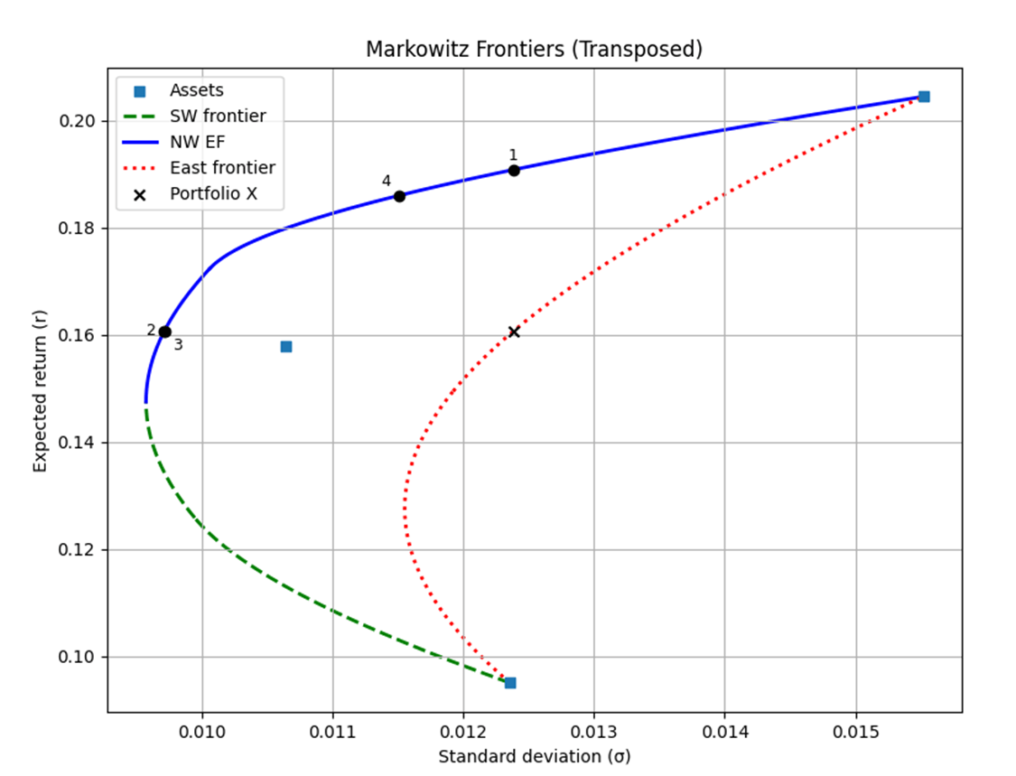

=== Portfolio Diagnostics ===
Portfolio r_w = 0.16064
Portfolio sd_w = 0.012384990916427835
Portfolio w  = [0.6, 0.0, 0.4]
1) Frontier at same variance (same sd as w):
   frontier source = EF
   r_frontier      = 0.19075250864468404
   r_diff          = 0.03011250864468404
   dissimilarity D = 0.3999999999999987
2) Frontier at same return r_w:
   frontier source = EF
   sd_frontier     = 0.009714263423226663
   sd_diff         = 0.002670727493201172
   dissimilarity D = 0.6395367908104868
3) Nearest EF point in (r, sd) space:
   r_ef            = 0.16069641602984358
   sd_ef           = 0.009715453211638733
   r_diff          = 5.641602984357563e-05
   sd_diff         = -0.0026695377047891017
   distance        = 0.0026701337655095064
   dissimilarity D = 0.6397796590869596
4) Closest EF point in WEIGHT space (min D):
   r_ef            = 0.1859313443141879
   sd_ef           = 0.011507702823987553
   r_diff          = 0.02529134431418789
   sd_diff         = -0.0008772880924402815
   dissimilarity D = 0.3999999999999987
=== Weight Details (w_deltas=True) ===
[1] w_f & Δw to same-variance frontier:
   w_f: [0.7065055622512704, 0.29349443774872697, 0.0]
   Δw:  [0.10650556225127039, 0.29349443774872697, -0.4]
[2] w_f & Δw to same-return frontier:
   w_f: [0.23229557457057015, 0.6395367908104864, 0.12816763461894287]
   Δw:  [-0.3677044254294298, 0.6395367908104864, -0.27183236538105715]
[3] w_f & Δw to nearest EF (r,sd) portfolio:
   w_f: [0.2326716222419909, 0.6397796590869593, 0.12754871867104933]
   Δw:  [-0.3673283777580091, 0.6397796590869593, -0.2724512813289507]
[4] w_f & Δw to closest-in-weights EF portfolio:
   w_f: [0.6028246089072669, 0.3971753910927305, 0.0]
   Δw:  [0.002824608907266879, 0.3971753910927305, -0.4]
============================

What does all of the above tell us? Let’s start with the graph. The blue line represents the lowest variance possible at the highest returns. The green line identifies the lowest variance at that the lower returns and the red line represents the highest variance at all returns. Together, they create the contours of the portfolio cloud – all of the possible return-variance pairs that were possible. The Boxes represent the assets, the X represents my specific allocation, and the black dots refer to the below diagnostics.

The output identifies the highest return that I could have achieved while keeping the portfolio variance constant. It also reports the difference between reality and that higher return. The above output says that my portfolio didn’t do too badly. I could have borne the same risk and achieved 3pp greater return. Finally, it reports the gross allocation changes that would have closed the gap – 40% of my portfolio would have needed to change. Ouch, that’s not flattering
It also identifies the lowest standard deviation that I could have achieved while keeping the return constant. again with the difference between reality and that lower standard deviation. The above output says that my portfolio sd was 0.0124 and could have been 0.0097 without sacrificing return. I was bearing 27% more volatility than I needed to in order to reach the same return. Further, I would have selected my allocations at least 64% differently in order to do it. Of all the numbers, it’s this minimally necessary change in weights that hurts the most. It’s a practical measure of your wrong decision.
This 3^rd stat is less useful, it identifies the nearest point on the return-maximizing & variance minimizing curve. Given that the sd is almost always less than the return, it tends to yield a very similar result as diagnostic 2).
Finally, the last diagnostic describes the portfolio on the efficient frontier that you could have achieved with the minimal change in portfolio weights. It’s a measure of “what’s the closest you were to doing things right?” It turns out that I could have had both higher returns and lower volatility if I have adopted a different mix of the same assets. Specifically, if I had changed my exposures by 40%, then I’d have been better off.

The function also yields the weight details in each case. For each of the 4 diagnostics, the weight details report the asset weights of the frontier portfolio for 1-4, and also report how the weight of each specific asset in your portfolio would have needed to be different.

For savvy users, the function can also optionally report the piece-wise quadratic functions that describe the efficient frontier. But I leave that as an exercise for the reader.

Financiers usually evaluate portfolios in terms of how much more return or how much less variance was left on the table. But I prefer to identify how the allocation – the choice variable – differed from the alternatives. This provides concrete feedback about what could have, and maybe should have, been done differently.

—

BTW, I’m the author of the above python function. You can find it on github here: https://github.com/zacharybartsch/frontier_segments