This post solves for the equilibrium quantity of production with quadratic total cost under Cournot and Stackelberg competition.
Say that there are two firms. They produce the exact same quality and type of goods and sell them at the same price. Let’s also assume that the market clears at one price. Finally, let’s assume increasing marginal costs.
Let’s say that they face the following demand curve:
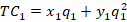
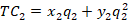
The firms have a total cost of:
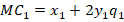
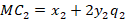
The marginal cost is the derivative with respect to the choice variable for each firm, or their respective quantities produced:
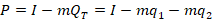
The total revenue is just the price times the quantity sold.


This is all standard fare for economic modeling. You’re free to make different assumptions. You can even adopt different slopes in the demand curve to reflect goods with different characteristics.
Cournot Competition
If you imagine a lengthy production process, or otherwise that they physically attend the same market, then it’s reasonable to assume that they don’t know one another’s choice of quantity produced.
We know how firms maximize profit: They produce the quantity at which the marginal revenue equals the marginal cost. But, what is marginal revenue? The derivative of total revenue with respect to the choice variable:
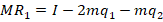
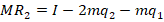
Now we can set the marginal revenue equal to marginal cost and solve for the optimal level of output:

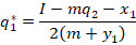

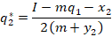
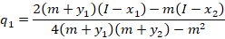
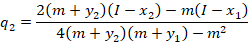
Notice that the optimal level of output depends on the production decision of the other firm. These are called response functions. If we solve for the quantities at which they intersect, then we are solving for where both firms are producing the best response to one another. This is known as a Pure Strategy Nash Equilibrium (PSNE).
Luckily, in many applications, one or more of the above terms are zeros, which makes things much simpler.
The general process for solving for the Cournot equilibrium is:
- Set MR=MC to find the response functions.
- Find where the response functions intersect.
