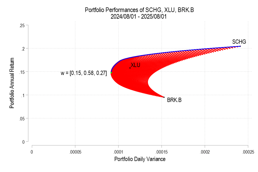
Previously, I plotted the possible portfolio variances and returns that can result from different asset weights. I also plotted the efficient frontier, which is the set of possible portfolios that minimize the variance for each portfolio return.* In this post, I elaborate more on the efficient frontier (EF).
To begin, recall from the previous post the possible portfolio returns and variances.


From the above the definitions we can see that the portfolio return depends on the asset weights linearly and that the variance depends on the asset weights quadratically because the two w terms are multiplied. Since the portfolio return can be expressed as a function of the weights, this implies that the variance is also a quadratic function of returns. Therefore, every possible portfolio return-variance pair lies on a parabola. So, it follows that every pair along the efficient frontier also lies on a parabola. Not every pair lies on the same parabola, however – the efficient frontier can be composed on multiple parabolas!
I’ll use the same 3 possible assets from the previous post, below is the image denoting the possible pairs, the EF set, and the variance-minimizing point.

One way to find the EF is to calculate every possible portfolio variance-return pair and then note the greatest return at each variance. That’s a discrete iterative process and it definitely works. One drawback is that as the number of assets can increase the number of possible weight combinations to an intractable number that makes iterative calculations too time consuming. So, we can instead just calculate the frontier parabolas directly. Below is the equation for a frontier parabola and the corresponding graph.


Notice that the above efficient frontier doesn’t appear quite right. First, most obviously, the portion below the variance-minimizing return is inapplicable – I’ve left it to better illustrate the parabola. Near the variance-minimizing point, the frontier fits very nicely. But once the return increases beyond a certain level, the frontier departs from the set of possible portfolio pairs. What gives? The answer is that the parabola is unconstrained by the weights summing to zero. After all, a parabola exists at the entire domain, not just the ones that are feasible for a portfolio. The implication is that the blue curve that extends beyond the possible set includes negative weights for one or more of the assets. What to do?
As we deduced earlier, each pair corresponds to a parabola. So, we just need to find the other parabolas on the frontier. The parabola that we found above includes the covariance matrix of all three assets, even when their weights are negative. The remaining possible parabolas include the covariance matrices of each pair of assets, exhausting the non-singular asset portfolios. The result is a total of four parabolas, pictured below.
