One of the major goals of the new Trump administration, particularly the DOGE unit, was to shrink the size of the federal government’s budget. Did they achieve this goal?
Last spring both my co-blogger Zachary and I pointed to a tool from the Brookings Institution to track federal spending, pulling in data directly from the US Treasury in a convenient format. Back in March I said “this will be a useful tool to follow going forward.” Now we have a full year of spending data for 2025.
When we look at total spending for Calendar Year 2025, it was about $318 billion higher than 2024, or about 4 percent higher. So, it seems that by that measure, the cuts that the Trump administration made were too small to overcome the other areas that grew.
But…
It may be more useful to remove some spending from the equation. In particular, entitlement programs and interest spending are very large spending categories that aren’t subject to the annual budgeting process. Of course, any program is ultimately under the control of Congress, so it’s a little bit of a cheat to remove Social Security and Medicare, but those programs are on autopilot with respect to the annual federal budget process. They are worth talking about, but they are probably worth talking about separately (especially because they have their own funding mechanisms). And interest on the debt isn’t something a President can control directly: it can only be reduced in future years by closing the budget gap today.
Removing those programs — which constitute about $4.8 trillion of the $7.9 trillion in 2025 spending (so a lot!) — gives you this chart (note: figures have been slightly updated with more complete data since I originally posted this chart):
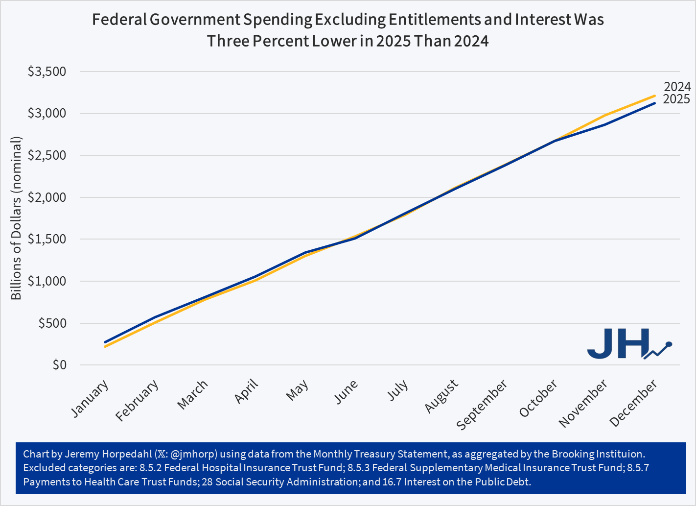
Federal spending by this measure was about $85 Billion lower in 2025 than the prior year, or about 5 percent. And that’s in nominal terms: it is an even bigger cut if we adjust for inflation. Notice too that the pattern fits what we might expect: spending was slightly higher in the first half of the year (before any Trump changes could have had much of an effect), almost exactly equal for most of the second half, and then slightly below once we get to November and December (after the Deferred Resignation Program layoffs in October). If we ignore the first two months of the year (when it would have been really hard for Trump to have an effect), the drop in spending is about 8 percent.
What were the biggest cuts that led to the $85 billion drop? Keep in mind that some programs increased spending, such as military spending, so there are more than $85 billion in cuts. Using the Daily Treasury Statement categories, here are the big ones:
- Federal Financing Bank (Treasury): $59 billion
- Department of Education: $46.8 billion
- USAID: $30.2 billion
- EPA: $17 billion (though EPA seems to have gone on a spending binge at the end of 2024. Compared with 2023, the first Trump year was 50% higher!)
- Federal Employee Insurance Payment (OPM): $16.3 billion
- Pension Benefit Guarantee Corporation: $11.3 billion
- Department of State: $8.6 billion
- Food Stamps (USDA SNAP): $4 billion
- CDC: $3.7 billion
- Crop Insurance Fund (USDA): $3.1 billion
- USDA Loan Payments: $2.7 billion
- Independent Agencies: $2.6 billion
- FCC: $1.8 billion
- NIH: $1.2 billion
- US Postal Service: $1.1 billion
Those are all the programs I could find that declined by at least $1 billion, totaling a little over $200 billion. There were some other highly salient cuts that were under a billion dollars (such as the Corporation for Public Broadcasting, which was completely eliminated). Looking at that list I don’t think there is an easy way to sum up a “theme,” but I think the real theme is that if the Trump administration wants 2026 discretionary spending to be even lower than 2025, they will really need some major action from Congress. These cuts are mostly low-hanging fruit, and some are long-running goals of the GOP (such as Dept. of Education, foreign aid, and public television).
Of course, to really get federal spending under control, Congress will have to tackle entitlement reform and shrink the budget deficit to lower interest costs. Social Security, Medicare, and interest payments — the bulk of federal spending, over 60% of the total — increase by 9% in 2025. Again, it was probably unreasonable to expect Trump and Congress to have done anything major with them in a single year, but something must be done soon: the Social Security Old Age trust fund will be depleted in about 8 years, and the Medicare Part A trust fund will be depleted in about 10 years.