My life didn’t change all that much due to Covid-19 pandemic. I live in a small university town. I mostly continued to go to work and my kids mostly continued to play with their neighbor friends. After a brief hiatus, I ended up growing much closer to my neighbors. One nearby couple are even the godparents my most recently born child.
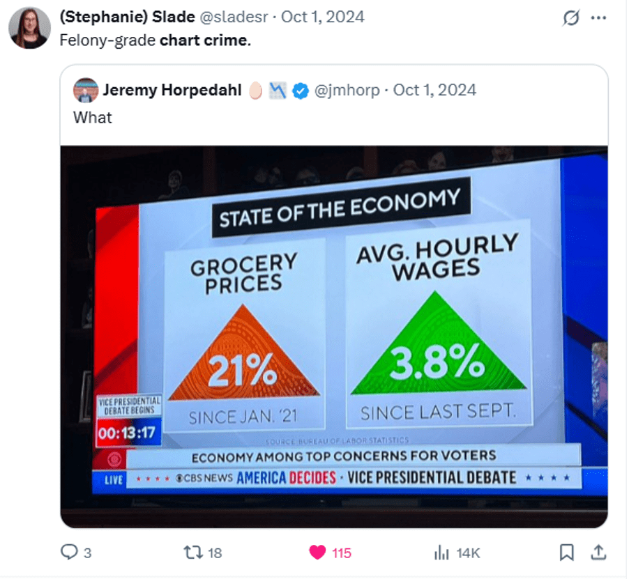
The university at which I teach is a liberal arts school…. And I teach economics. I knew that these music-type of students and professors were out there, but I didn’t have much exposure. I recently obtained a zero-priced piano and had a good 2-hour conversation with a music major. This post illustrates part of I’ve learned so far. First, a graph.
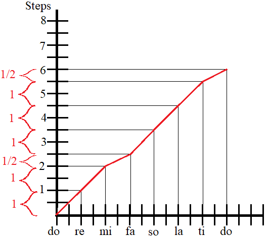
Whether we want to or not, many of us know the musical scale thanks to The Sound of Music. What I didn’t know was that there is not a uniform distance between all of those notes. Along the x-axis is the note labels (do re mi fa so la ti do). The pitch is characterized by an increment called a step. Given some arbitrary pitch for the first note, do, each subsequent note is a specific number of steps away. The pattern is that each increment between notes is 1 step, except the step from mi to fa and from ti to do. Those are half steps. The result is a segmented function.
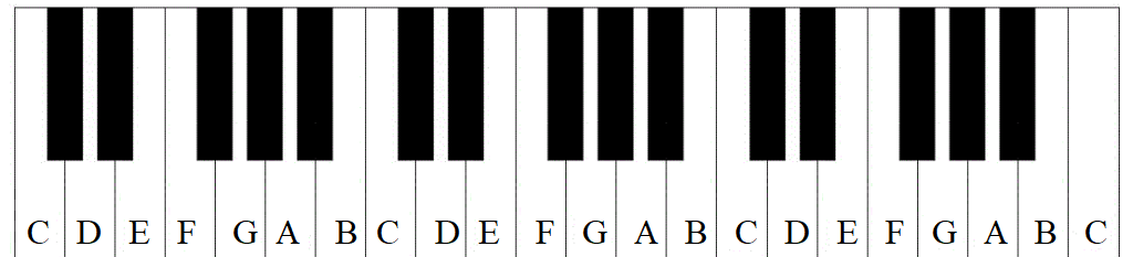
Now, this pattern can be applied to a piano.
There are a total of 88 keys on a piano. Some are black, others are white. But all of them are a half-step increment from the prior and subsequent key. IDK why there are small black keys and big white ones. But pianos would be a lot bigger without the narrower black keys. Every single white key on a piano is labeled with a letter. The letter *does not move*. A ‘C’ is always a ‘C’.
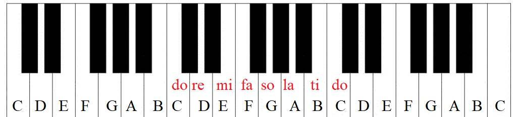
What can move is the scale label, do, which can be any key. The pattern identified in the graph above must be maintained. To play ‘in the key of C’ means that ‘C’ is identified as do. The remaining keys can be labeled.
The key of ‘C’ is easy because the entire scale can be played on all white keys.
Those two half steps that we mentioned earlier? Those might have been on a black key – except that there is no black key between ‘B’ and ‘C’ or between ‘E’ and ‘F’. The B-C keys are adjacent. That means that their pitch is a half-step apart – exactly what is necessary for the pitch difference between mi and fa. The same is true for the E-F step and the pitch difference between ti and do.
What about the black keys? We can see their roll by placing do on a different lettered key. We can start on ‘D’.
do to re is a full step, from ‘D’ to ‘E’ – skipping the black half-step that’s between them. For re to mi we need to skip a key, all keys are a half step apart. So? To the black key! We skip ‘F’ and land on the subsequent black key. Then, fa falls on ‘G’, a half step and a single key higher in pitch. ‘A’ is a full step away from ‘G’, so that’s so. la is another full step away on ‘B‘. Recall that all of the keys are separated by a half-step – the key colors are 100% unimportant. ti is a full step higher – but there is no key separating ‘B’ and ‘C’. So, we skip up to the black key again just as we did with mi. Finally, do is a single key and a half step more.
There you have it! One of the things that a pianists can do is play the entire scale, from do to do, starting from any lettered key on the piano. I can’t do that yet, but golly I certainly feel like I have a better handle of what I’m even looking at.
PS – My conversation took a long time and I had to nail down the difference between 1) The note label, 2) the pitch step increments, & 3) the piano key letter labels. Key letter labels and the note labels are ordinal variables while the steps are cardinal. So, the graph at the top of this post isn’t the only important relationship. The graph below includes the relationship between the step and key letter labels. A graph of the note label and the key letter labels requires a rudimentary knowledge of flats and sharps (with two different do’s).