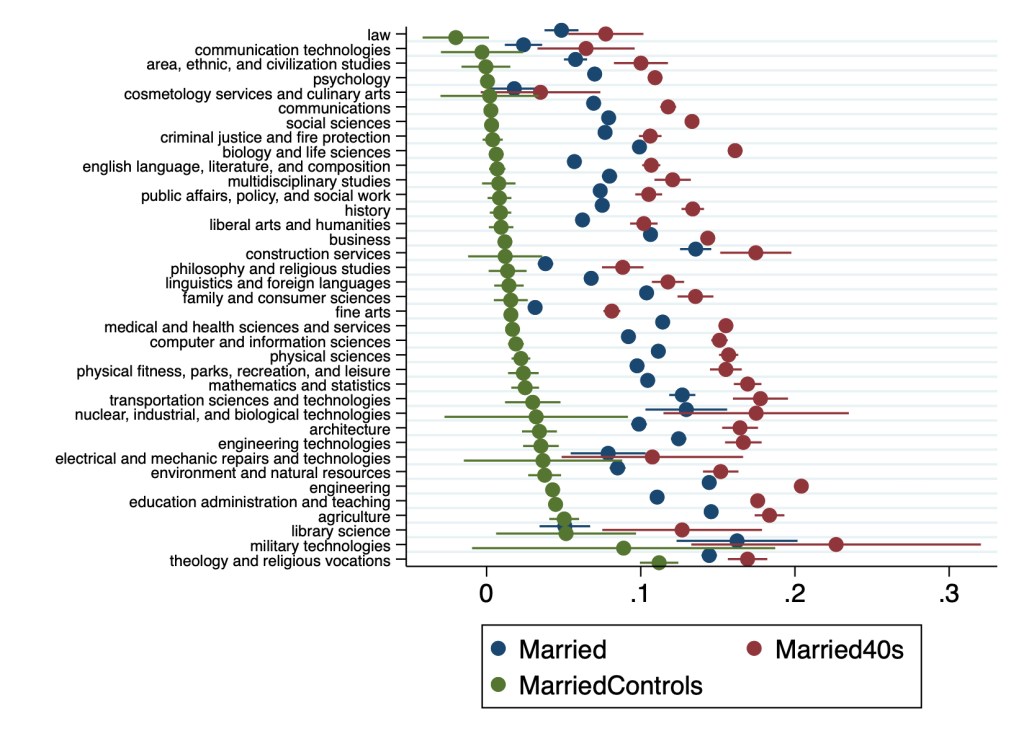
In a May post I described a paper my student my student had written on how college majors predict the likelihood of being married and having children later in life.

Since then I joined the paper as a coauthor and rewrote it to send to academic journals. I’m now revising it to resubmit to a journal after referee comments. The best referee suggestion was to move our huge tables to an appendix and replace them with figures. I just figured out how to do this in Stata using coefplot, and wanted to share some of the results:

Many details have changed since Hannah’s original version, and a lot depends on the exact specification used. But 3 big points from the original paper still stand:

1. Almost all majors are more likely to be married than non-college-graduates
2. The association of college education with childbearing is more mixed than its almost-uniformly-positive association with marriage
3. College education is far from uniform; differences between some majors are larger than the average difference between college graduates and non-graduates