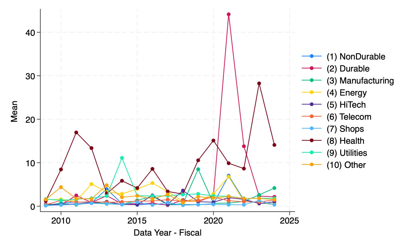
A reporter recently told me she thought there is a national trend toward hospitals issuing more bonds. I tried to verify this and found it surprising hard to do with publicly available data. But once I had to spend an hour digging through private Compustat data to find the answer, I figured I should share some results. Here’s the average debt in millions of companies by sector:
Source: My graph made from Compustat North American Fundamentals Annual data collapsed by Standard Industrial Classification code into the Fama-French 10 sectors
This shows that health care is actually the least-indebted sector, and telecommunications the most indebted, followed by utilities and “other” (a broad category that actually covers most firms in the Fama-French 10). But are health care firms really more conservative about debt, or are they just smaller? Let’s scale the debt by showing it as a share of revenue:
My graph made from Compustat North American Fundamentals Annual data collapsed by SIC code into the Fama-French 10 sectors(dltt/revt).
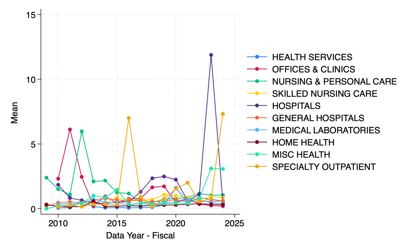
It appears that health care firms are the most indebted relative to revenue since 2023. But which parts of health care are driving this?
Hospitals in 2023 followed by specialty outpatient in 2024. However, seeing how much the numbers bounce around from year to year, I suspect they are driven by small numbers of outlier firms. This could be because Compustat North America data only covers publicly traded firms, but many sectors of health care are dominated by private corporations or non-profits.
I welcome suggestions for datasets on the bond-market side of things that are able to do industry splits including private companies, or suggestions for other breakdowns you’d like to see me do with Compustat.
This post is co-written with John Olis, History major at Ave Maria University.
There is a popular myth that manufacturing jobs of the past provided a leg-up to young people. The myth goes like this. Manufacturing jobs had low barriers to entry so anyone could join. Once there, the job paid well and provided opportunities for fostering skills and a path toward long-term economic success. There is more to the myth, but let’s stop there for the moment. Is the myth true?
One of my students, John Olis, did a case study on Connecticut in 1920-1930 using cross sectional IPUMS data of white working age individuals to evaluate the ‘Manufacturing Myth’. We are not talking causal inference here, but the weight of the evidence is non-zero. The story above has some predictions if not outright theoretical assertions.
Manufacturing jobs paid better than non-manufacturing jobs for people with less human capital.
Manufacturing jobs yielded faster income growth than non-manufacturing jobs.
Implicitly, manufacturing jobs provided faster income growth for people with less human capital.
Using only one state and two decades of data obviously makes the analysis highly specific. Expanding the breadth or the timescale could confirm or falsify the results. But historical Connecticut is a particularly useful population because 1) it had a large manufacturing sector, 2) existed prior to the post WWII boom in manufacturing that resulted from the destruction of European capacity, and 3) had large identifiable populations with different levels of human capital.
Who had less human capital on average? There are two groups who are easy to identify: 1) immigrants and 2) illiterate people. Immigrants at the time often couldn’t speak English with native proficiency or lacked the social norms that eased commercial transactions in their new country (on average, not always). Illiterate people couldn’t read or write. Therefore, having a comparative advantage in manual labor, we’d expect these two groups to be well served by manufacturing employment vs the alternative.
Being cross-sectional, the individuals are not linked over time, so we can’t say what happened to particular people. But we can say how people differed by their time and characteristics. Interaction variables help to drill-down to the relevant comparisons. There are two specifications for explaining income*, one that interacts manufacturing employment with immigrant status and one that interacts the status of illiteracy. The baseline case is a 1920 non-operative native or literate person. Let’s start with the below snapshot of 1920. The term used in the data is ‘operative’ rather than ‘manufacturer’, referring to people who operate machines of one sort or another. So, it’s often the same as manufacturing, but can also be manufacturing-adjacent. The below charts illustrate the effect of lower human capital in pink and the additional subpopulation impacts of manufacturing in blue.
In the left-hand specification, native operatives made 2.2% less than the baseline population. That is, being an operative was slightly harmful to individual earnings. Being an immigrant lowered earnings a substantial 16.8%, but being an operative recovered most of the gap so that immigrant operatives made only 6.1pp less than the baseline population and only 3.9pp less than native operatives. In the right-hand specification, unsurprisingly, being illiterate was terrible for one’s earnings to the tune of 23.4pp. And while being an operative resulted in a 1.2% earnings boost among natives, being an operative entirely eliminated the harm that illiteracy imposed on earnings.
Both graphs show that manufacturing had tiny effects for a typical native or literate individual. But manufacturing mattered hugely for people who had less human capital. So, prediction 1) above is borne out by the data: Manufacturing is great for people with less-than-average human capital.
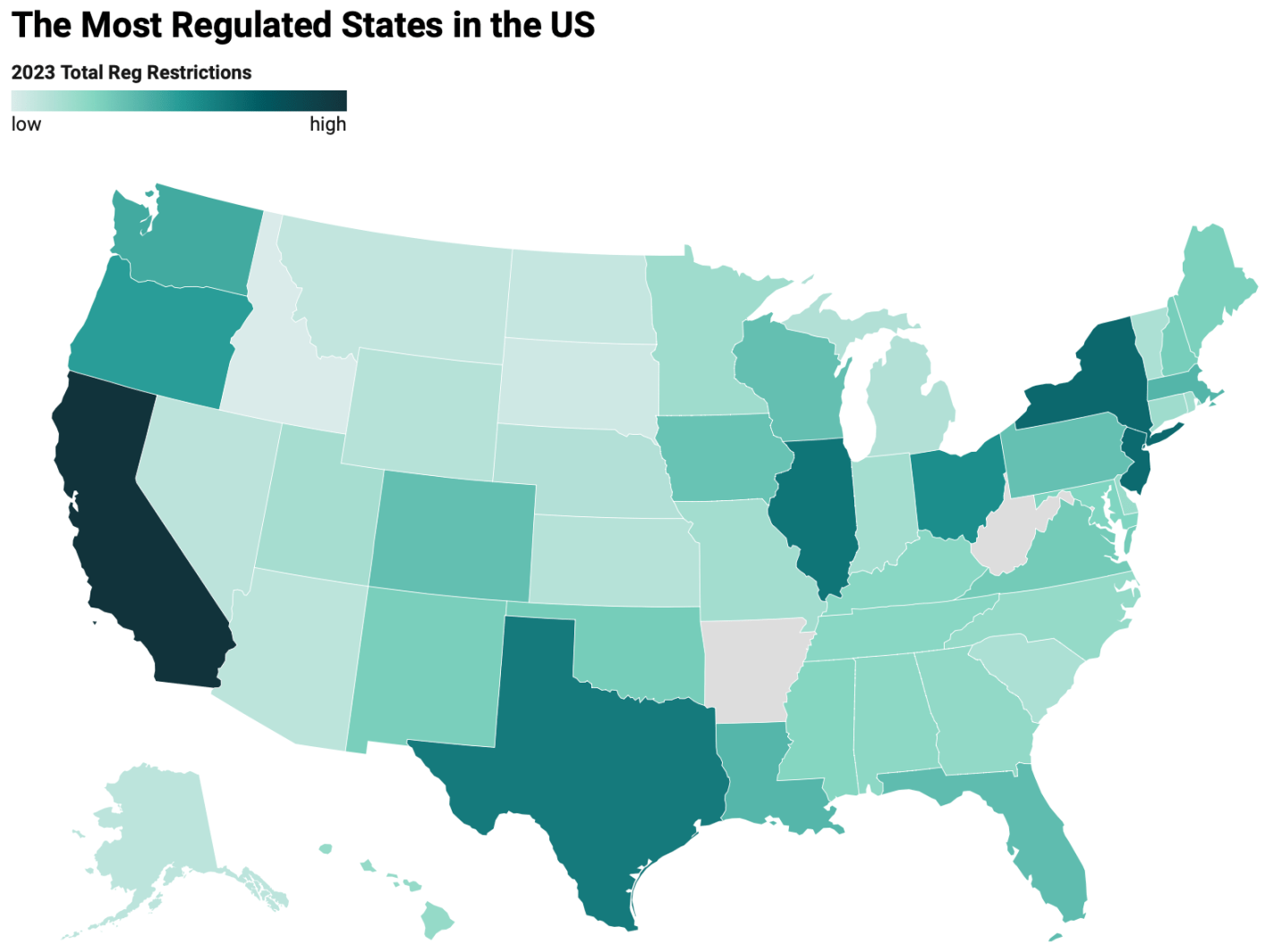
The Mercatus Center has put together a page of “Snapshots of State Regulation” using data from their State RegData project. Their latest data suggests that population is still a big predictor of state-level regulation, on top of the red/blue dynamics people expect:
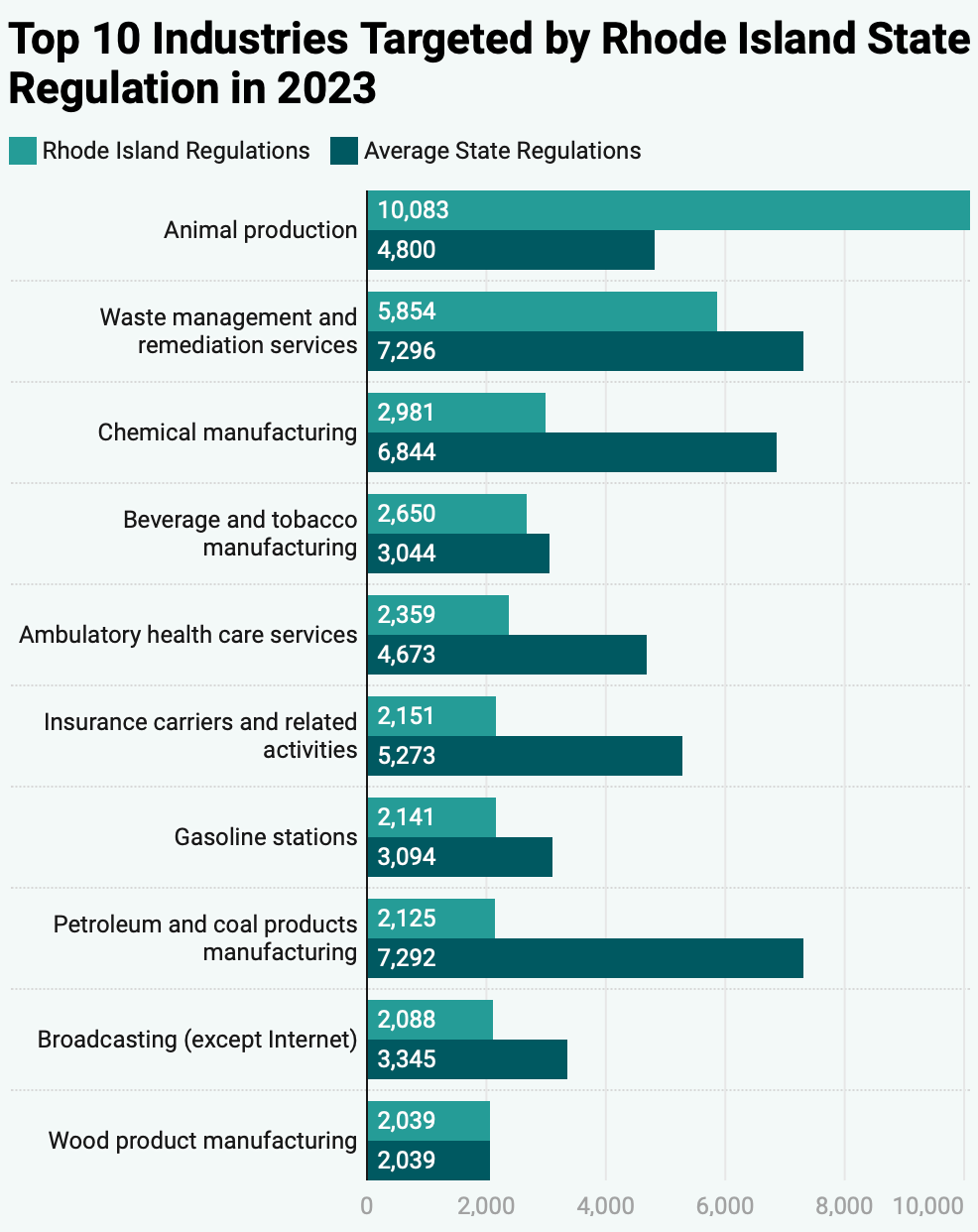
They also made pages with much more detail on each state, like what the most regulated industries in each state are and how each one compares to the national average:
Has it gotten easier or harder for Americans to afford the basic necessities of life? Part of the answer to this question depends on how you define “basic necessities,” but using the common triad of food, clothing, and housing seems like a reasonable definition since these composed over 80% of household spending in 1901 in the United States.
If we use that definition of necessities, here is what the progress has looked like in the US since 1901:
The data comes from various surveys that the Bureau Labor Statistics has collected over the years, collectively known as the Consumer Expenditure Surveys. The surveys were conducted about once every 1-2 decades from 1901 up until the 1980s, and then annually starting in 1984. Some of these are multi-year averages, but to simplify the chart I’ll just state one year (e.g., “1919” is for 1918 and 1919). The categories are fairly comprehensive: “food” includes both groceries and spending at restaurants; “housing” includes either mortgage or rent, plus things like utilities and maintenance; and “clothing” includes not only the cost of the clothes themselves, but services associated with them such as repairs or alterations (much more important in the past).
We can see in the chart that over time the share spent on these three areas of spending has declined dramatically, taken as a group. Housing is different, but it has been fairly stable over time, mostly staying between 22% and 29% of income (the Great Depression being an exception). There are two time periods when these costs rose: the Great Depression and the late 1970s/early 1980s. Both are widely recognized as bad economic times, but they are aberrations. The jump from 1973 to 1985 in spending on necessities was fully offset by 2003, and today spending on necessities is well below 1973 — even though for housing, it is a few percentage points greater.
A chart like this shows great progress over time, but it will inevitably raise many questions. Let me try to answer a few of them in advance.
I just learned about the Bayesian Dawid-Skene method. This is a summary.
Some things are confidently measurable. Other things are harder to perceive or interpret. An expert researcher might think that they know an answer. But there are two big challenges: 1) The researcher is human and can err & 2) the researcher is finite with limited time and resources. Even artificial intelligence has imperfect perception and reason. What do we do?
A perfectly sensible answer is to ask someone else what they think. They might make a mistake too. But if their answer is formed independently, then we can hopefully get closer to the truth with enough iterations. Of course, nothing is perfectly independent. We all share the same globe, and often the same culture or language. So, we might end up with biased answer. We can try to correct for bias once we have an answer, so accepting the bias in the first place is a good place to start.
The Bayesian Dawid-Skene (henceforth DS) method helps to aggregate opinions and find the truth of a matter given very weak assumptions ex ante. Here I’ll provide an example of how the method works.
Let’s start with a very simple question, one that requires very little thought and logic. It may require some context and social awareness, but that’s hard to avoid. Say that we have a list of n=100 images. Each image has one of two words written on it, “pass” and “fail”. If typed, then there is little room for ambiguity. Typed language is relatively clear even when the image is substantially corrupted. But these words are written, maybe with a variety of pens, by a variety of hands, and were stored under a variety of conditions. Therefore, we might be a little less trusting of what a computer would spit out by using optical character recognition (OCR). Given our own potential for errors and limited time, we might lean on some other people to help interpret the scripts.
Claims that the middle class or working class has been “hollowed out” in the US have been made for years, or decades really. The latest claim is an essay in the Free Press by Joe Nocera. But these claims are usually lacking in data, while strong in anecdotes. Let’s look at the data.
Notice that the latest data point is for 2024, which is the highest they have ever been in this data series, and likely higher than any point in the past. While many point to about the year 2000 as when troubles for the working class started (this is when manufacturing employment really fell off a cliff, and China joined the WTO in 2001), inflation-adjusted earnings have risen 11% for this group of workers since then. You might say that’s not a lot of growth — and you would be correct! But this group is better off economically than in the year 2000, which is a point that gets lost in so many discussions about this issue.
But that’s just a national number. Might some states that were especially hit by manufacturing job losses be worse off? Nocera mentions North Carolina and the Midwest. To answer this, we can use BLS OEWS data, which has not only median wages by state, but also the 10th percentile wage — the lowest of the working class. Here’s what median real wage growth (again inflation-adjusted with the PCEPI) since 2001 (the earliest year in this series with comparable data):
There was a recent Planet Money Podcast episode that includes a fun exercise. An NPR employee produces a dozen chicken eggs and wants to sell them at cost to another employee for $5. That’s the setup. How does the employee decide who should receive the eggs? Clearly, the price mechanism won’t work since the price is fixed. A lottery is also not allowed. The egg recipient could engage in arbitrage, reselling the eggs for a higher price. But that’s not very likely and would be socially awkward. The egg producer wants to make someone happy. Who would he make the happiest?
That’s the challenge that the Planet Money team tries to solve.
First, they started with a survey. Rather than asking coworkers to rank a long list of things that includes eggs, the survey adopts a more robust method of pairwise comparisons. Do you prefer toast vs eggs? Eggs vs oatmeal? Toast vs oatmeal? and so on. One problem that they encounter, however, is that there is a lot of diversity among preparations methods. My oatmeal is better than my eggs. But my brother’s oatmeal is not. As it turns out, there is not a standard quality of prepared oatmeal and prepared eggs. So the survey is a flop.
Then they consult an economist. They decide to try to measure “willingness to pay”, which is an economic concept that identifies the maximum that a person could pay for something without becoming worse off. They couldn’t really ask the coworkers what their WTP is. People are social creatures and have many reasons to lie, mislead, signal, and to simply not know. Since someone’s WTP reflects preferences and values, we need a way to solicit the true preference while avoiding lies and most mistakes. Here’s how the economist suggested that they reveal the coworker preferences.
Step 1: Tell the coworker these rules.
Step 2: Coworker reports their WTP for a single egg in dollars
Step 3: A random price will be chosen by a machine. If the price is above the self-reported WTP, the coworker is not allowed to buy the egg. If the price is below the WTP, then the coworker must buy the egg at the random price.
I like to take existing datasets, clean them up, and share them in easier to use formats. When I started doing this back in 2022, my strategy was to host the datasets with the Open Science Foundation and share the links here and on my personal website.
OSF is great for allowing large uploads and complex projects, but not great for discovery. I saw several of my students struggle to navigate their pages to find the appropriate data files, and they seem to have poor SEO. Their analytics show that my data files there get few views, and most of the ones they get come from people who were already on the OSF site.
This year I decided to upload my new projects like County Demographics data to Kaggle.com in addition to OSF, and so far Kaggle is the clear winner. My datasets are getting more downloads on Kaggle than views on OSF. I’ve noticed that Kaggle pages tend to rank highly on Google and especially on Google Dataset Search. I think Kaggle also gets more internal referrals, since they host popular machine learning competitions.
Kaggle has its own problems of course, like one of its prominent download buttons only downloading the first 10 columns for CSV or XLSX files by default. But it is the best tool I have found so far for getting datasets in the hands of people who will find them useful. Let me know if you’ve found a better one.
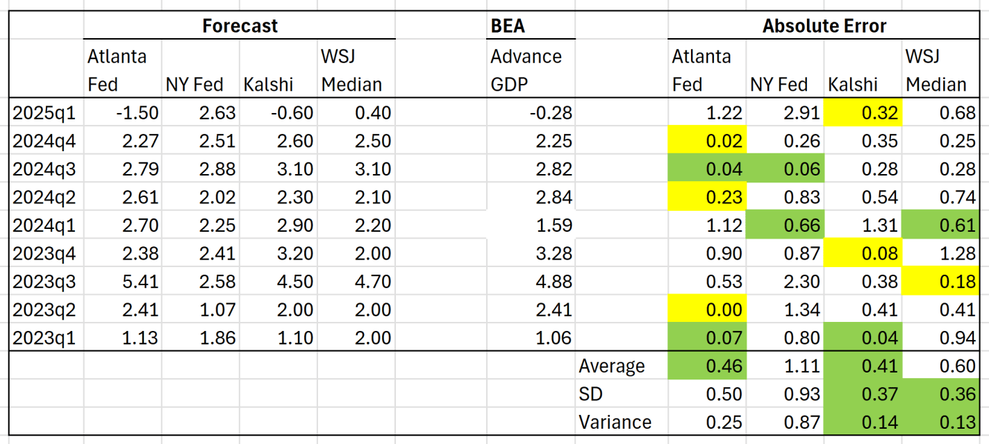
The 2025 first quarter GDP data came in slightly bad: negative 0.3%. I think the number is a bit hard to interpret right now, but it’s hard to spin away a negative number. A big factor pulling down the accounting identify that we call GDP was a massive increase in imports, specifically imports of goods. It’s likely this is businesses trying to front-run the potential tariffs (and keep in mind this was pre-“Liberation Day,” so probably even more front running in April), so the long-run effect is harder to judge.
But aside from the interpretation of the GDP estimate, we can ask a related question: did anyone predict it correctly? I have written previously about two GDP forecasts from two different regional Federal Reserve banks. They were showing very different estimates for GDP!
Both the Fed estimates ending up being pretty wrong: -1.5% and +2.6%. But there are two other kinds of forecasts we can look at.
The first is from a survey of economists done by the Wall Street Journal. The median forecast in that survey was positive 0.4%. This survey got the direction wrong, but it was much closer than the Fed models.
Finally, we can look at prediction markets. There are many such markets, but I’ll use Kalshi, because it’s now legal to use in the US, and it’s pretty easy to access their historical data. The average Kalshi forecast for Q1 (a weighted average of sorts across several different predictions) was -0.6%. Pretty close! They got the direction right, and the absolute error was smaller than WSJ survey. And obviously, much better this quarter than the Fed models.
But this was just one quarter, and perhaps a particularly weird quarter to predict (Atlanta Fed even had to update their model mid-quarter, because large gold inflows were throwing of the model). You may say that weird quarters are exactly when we want these models to perform well! But it’s also useful to look at past predictions. The table below summarizes predictions for the past 9 quarters (as far back as the current NY Fed model goes):
Generally, decisions to spend federal funds come is the authority of congress. But the Trump administration has very publicly made clear that it will try to cut the things that are within its authority (or that it thinks should be within that authority). Truly, the fiscal year with the new Republican unified government won’t begin until October of 2025. So, the last quarter is when we’ll see what the Republicans actually want – for better or for worse. In the meantime, we can look past the hyperbole and see what the accounting records say. The most recent data includes 95 days after inauguration. First, for context, total spending is up $134 billion or 5.8% from this time last year to $2.45 trillion.
The Trump administration has been making news about their desire and success in cutting. Which programs have been cut the most? As a proportion of their budgets, below is a graph of were the five biggest cuts have happened by percent. The Cuts to the FCC and CPB reflect long partisan stances by Republicans. The cuts to the Federal Financing Bank reflect fewer loans administered by the US government and reflect the current bouts to cut spending. Cuts in the RRB- Misc refer to some types of railroad payments to employees. In the spirit of whiplash, the cuts to the US International Development Finance Corporation reverse the course set by the first Trump administration. This government corporation exists to facilitate US investment in strategically important foreign countries.
But some programs have *increased* spending since 2024. The five largest increases include the USDA, the US contributions to multilateral assistance, claims and judgments against the US, the federal railroad administration, and the international monetary fund. Funding for farmers and railroads reflect the old agricultural and new union Republican constituencies. The multilateral assistance and IMF spending reflects greater international involvement of the administration, despite its autarkic lip service.