A Measure of Dissimilarity

I recently learned about an interesting statistic for social scientists. It’s called the “Dissimilarity Index”. It allows you to compare the categorical distribution of two sets.

Many of us already know how to compare two distributions that have only 2 possible values. It’s easy because if you know the proportion of a group who are in category 1, then you know that 1-p will be in category 2. We can conveniently denote these with values of zero and one, and then conduct standard t-tests or z-tests to discover whether they are statistically different. But what about distributions across more than two possible categories?

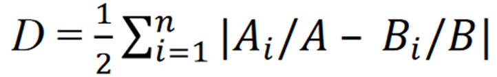
Enter the dissimilarity index (DI). Once you have the proportion of 2 groups who are in each category, sum the absolute values of their halved differences. What does it yield? It yields the proportion of people who would need to change categories in order for the two groups to be identically distributed across the categories. For example, a DI value of 0.32 means that 32% of the total proportional change would make the two groups identical. The equation is below.

How is it useful? Well, you can measure whether the categorical distribution of two groups is big or small. Then, you can measure whether they become more or less similar over time.

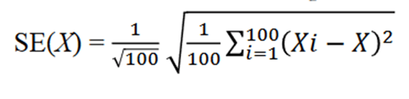
And, no statistic would be complete without a method of calculating a p-value. First, we’d calculate a standard error (SE). To do that, you just split your 2 groups up into 100 random samples. Then, you calculate the DI, and then the Subsample DI’s squared difference from the original DI. Then, you average them, take the square root, and divide by 10. The result is a nice familiar SE. Here’s the equation:

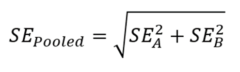
The ratio of the DI and the SE yields a test statistic that is asymptotically normal – which means that you can treat them the same way that you would a Z-statistic. Badda-bing badda-boom, there’s a p-value associated with that Z. That means that you can say: 1) How dissimilar (or similar) two categorical distributions are, and 2) how confident we should be in their difference. Further, by calculating the DI at two points in time, we can use a good old-fashioned pooled SE in order to say 3) whether the change over time is significant.

Nifty!

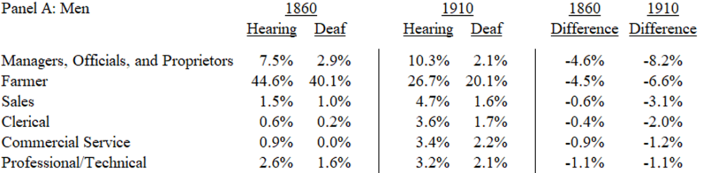
Here’s an application. Below is a table that illustrates part of the occupational distribution of hearing and deaf males in 1860 and 1910. Look at 1860. Sure, the distributions are different – maybe even dissimilar. But are they significantly dissimilar? Now we can say! The 1860 DI was 0.143 (SE=0.014) and the 1910 DI was 0.222 (SE=0.013). Those are both very different from zero. With the pooled SE, we can say that dissimilarity between deaf and hearing worker occupations increased by 0.079 (SE=0.019). Plenty of things were happening in that 50 year period that could have cause the increasing dissimilarity. It could have been technological change, such as the spread of telephones, or it could have been educational, such as the popularization of teaching oral communication and the suppression of sign language. Whatever was happening in the intervening 50 years, it sure wasn’t making deaf workers more similar to hearing workers. Which, of course, isn’t particularly desirable in itself. But, given that deaf workers tended to have lower earnings, it seems like something worth investigating further.

*A clear use case of the statistic is in the below paper, which clearly lays out an application and includes the top two equations.

Liebler, Carolyn A., Jacob Wise, and Richard M. Todd. 2018. “Occupational Dissimilarity between the American Indian/Alaska Native and the White Workforce in the Contemporary United States.” American Indian Culture and Research Journal 42 (1). https://doi.org/10.17953/aicrj.42.1.liebler.