Say that you have a bachelor’s in finance, but that you’re not exactly a ‘math’ person. You know that diversification is good for reducing the volatility of returns, but the calculations are a bit mysterious to you. You know what the efficient frontier is, but its calculation is elusive. All is not lost! There are alternatives to the math: Sampling methods. By testing a few possible portfolios, we can get an idea of which one is the best fit for you. Here I’ll provide an example using 1) a simple random sample, 2) stratified random sample, 3) Sobol sequence, & 4) Scrambled Sobol.
I’ll use a two-asset portfolio here for ease. I assume that the portfolio includes no short or leveraged positions and that the asset weights sum to one. This is known as ‘long only’. The challenge is that we want a certain return-volatility profile for our portfolio, but it’s a bit hard to figure out what our options are. Luckily, both return and standard deviation (SD) of a portfolio are determined by the weights on the individual assets.
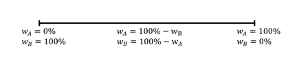
With a long only portfolio, all possible weights are uniformly distributed between one asset having zero weight and the same asset having 100% of the weight. Since the weights sum to one, whatever weight remains after the first asset is attributable to the 2nd asset. See the figure below. Unlike many distributions, we know exactly what’s possible for the weights. The portfolio expected return is simply the linearly weighted average and the portfolio variance is quadratically weighted. Return and SD equations are below.
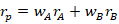

The portfolio return is mathematically easy, since it’s just a linear average: more weight on asset A implies a rate of return that is closer to that of asset A. But the same is not true for SD, due to the covariance component. We can graph how both portfolio returns and SD are related to the asset weights below.
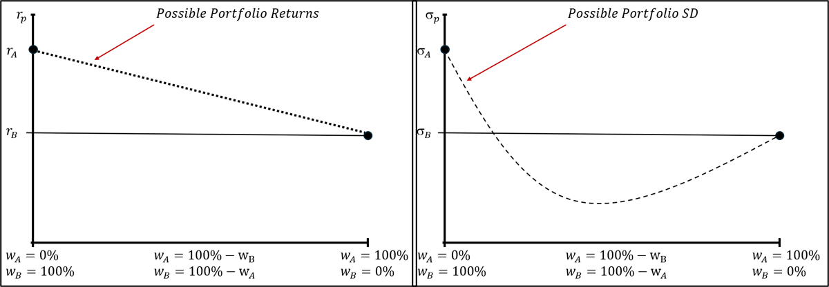
We already know that the possible weights are distributed uniformly (and so are the returns), but the possible SD are not distributed uniformly. Without the math, we want to know what our possible portfolio SD are so that we can determine what mix of assets is right for us. This example is a bit trite, but the gains occur when generalizing to many-asset portfolios. We can choose from a few methods for describing the correspondence between weights and the SD.
Method 1: Random Sample
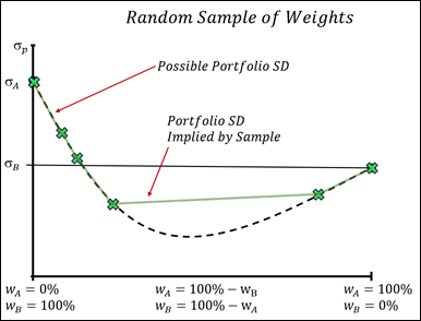
The easiest thing to do is take a random draw of a few weights and calculate their associated returns and SDs. However, randomness also implies that we may get a set of points which are clustered together or that don’t sample the various nooks and crannies very well. An example of a random sample is below, along with a line that connects the sampled options (I assume that we know the extrema weights: 0% & 100% values). Random sampling does an ‘ok’ job of choosing relevant portfolio allocations. But due to the random nature, substantial pieces of the actual SD menu options may be omitted. Sometimes the omitted portions are no big deal and other times they are – and which occurs entirely at random. In the image below, the random portfolios left out the possible allocations that yielded the lowest volatility.
Method 2: Stratified Random Sample
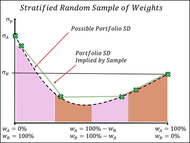
The fact that the possible weights are distributed uniformly in weight-space is a big advantage. One way to constrain our sample of weights is to use a stratified random sample. In this case, we split the uniform weights into several equal intervals and then take a random sample from within each interval. This ensures that each interval’s characteristics are reflected, even partially, in the overall sample. The various shaded regions below reflect the regions from which a sample was drawn. While the regions are uniformly distributed, the random sample(s) within each region can occur anywhere within the region.
The green line implied by the sample is closer to the minimum SD, and the portions that have less weight on asset A are now less accurate (further from the dotted line). So, we gained some precision in some parts of the SD correspondence, but lost some in others. Loss is especially likely to occur near more jagged or irregular possible values. Since we don’t necessarily want the minimum SD allocation, using a stratified random sample is not always better than a simple random sample. But at least the maximum gaps between the observations are constrained. A simple random sample can detect local irregular shape sometimes, whereas a stratified random sample might always lack adequate resolution in a narrow interval.
Method 3: Sobol Sequence
Rather than the random draws that characterize the simple random sample or the stratified random sample, we can just adopt a deterministic sequence of weights to evaluate. A Sobol sequence, or just ‘Sobol’, draws weights at equal intervals – which is perfect for the uniformly distributed possible weights and is often best for characterizing a function (SD in this case)**. Specifically, the Sobol observes the weights at increments up to each power of ½ (1/4, 1/8, 1/16…) and includes zero by default. So, below, with 4 observations, the weights of asset A occur at (0, 0.25, 0.5, 0.75). Just like the random methods, I’ll toss in the endpoints for free since they’re already known. Note that this means we have fewer observations with the Sobol because it would have grabbed the asset A weight of 0 regardless.
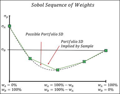
A nice characteristic of a Sobol is that the observations are equally spaced apart. That means that there is no error due to the variation in gaps between the sequenced weights – nor randomness otherwise. In the above image, the observed weights get close to the minimum SD weight and the green line closely approximates the true line. It performs better than the stratified random sample of weights *despite* evaluating one less observation. The number of Sobol sequence observations is entirely at the discretion of the desired resolution. For a stratified random sample, the number of strata *must* scale with the number of dimensions. If you have computationally intensive processes, then a Sobol can save a lot of resources – especially when the modeled function is deterministic such as for portfolio SD.
Method 4: Scrambled Sobol
The final option that I cover is the Scrambled Sobol. Similar to the simple Sobol sequence, it breaks up the possible weights into 4 equal intervals. Then, randomly decides from which half of that interval to sample. Then, it decides randomly which sub-interval to sample, ad infinitum. In applications, it stops this process at bit-precision.
When there is only 1 dimension, such as in our 2-asset portfolio where a single weight characterizes all other weights, the result is identical to the Stratified Random Sample. The advantages of the Sobol and scrambled Sobol are more pronounced in high-dimension problems. The resolution is what we want it to be. Further, adding more data requires that stratified random sample be recalculated and sampled, whereas a Sobol can reuse the prior observations and sequence more observations for the new data.
Finally, a stratified sample creates a grid over all possible weights, and that grid includes a lot of repeating values that don’t add additional information. After all, one or two assets might have any fixed weight. Then, we could vary other weights and we wouldn’t need to keep sampling the ones that are constant locally. So, the Sobol can achieve similar SD resolution with fewer sequenced weights.
The primary benefit of any Sobol is that it performs well with a higher number of dimensions (more assets). A related benefit concerns percentiles. If you want to know how many other possible SD a particular portfolio ‘beats’, then can both Sobols can yield a percentile – and the scrambled Sobol can yield a standard error for that percentile. A stratified random sample can do the same, but requires many more observations with increased dimensionality.
**Any sequence size is possible. And the density of observed weights will stay uniform so long as N=2^m, where m number of halvings that describe the observation intervals. Otherwise, the density of the observations will be irregular for some weight domains.

