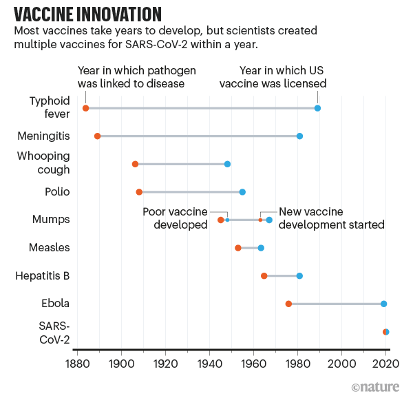
We’ve already talked about different methods for distributing the vaccine in the face of limited supply on this blog (see my post and Doug Norton’s post). But today I want to talk about something different: the speed at which this vaccine was developed. It is truly amazing.
This chart from Nature (adapted from the fantastic Our World in Data) dramatically shows just how quickly the COVID-19 vaccine was developed compared with past vaccines. What used to take decades or even a century was done in mere months (yes, even with all the regulatory barriers today).
Exactly how we developed this vaccine so quickly is a complex story that involves the advanced state of modern science, incentives offered by concerned governments, and the harnessing of the profit motive to advance the public good. We don’t know all the details yet, and likely won’t for a long time since, like a pencil, no one person knows how to make and distribute a vaccine.
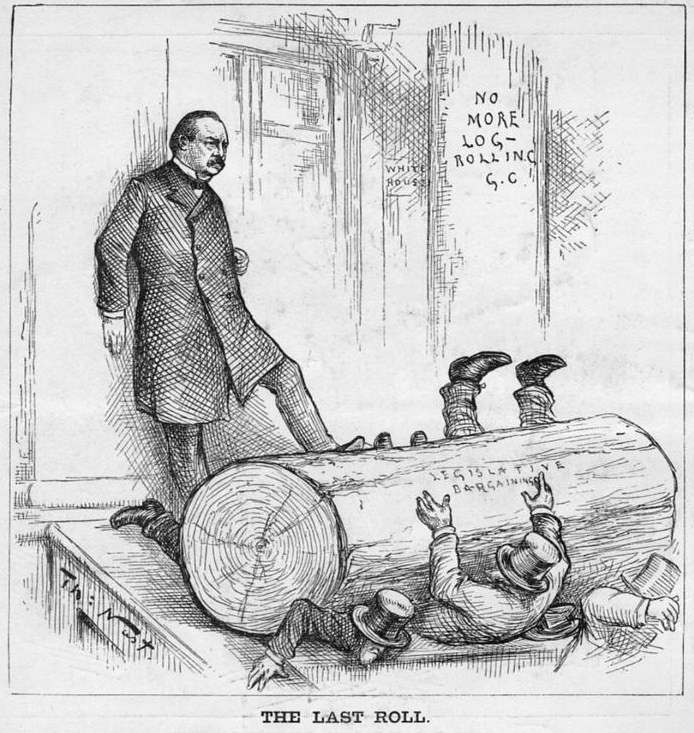
Along with the colorful phrase “pork barrel” spending, logrolling is a term used to describe the process of vote trading in elected legislative bodies. The process has long been maligned by political scientists, pundits, and the general public. It’s also come up in the debate about the proposed Budget/COVID Relief Bill.
President Grant tried to stop logrolling. He failed.
What’s bad about logrolling? I think there are two general lines of argument. First, it just seems immoral. Citizens can’t legally trade their votes, and many see any attempt to do so as wrong. You get one vote, and one vote only. For someone to have more votes than others rubs our intuitions the wrong way, similar to the ability for wealthy individuals or corporations to essentially have more votes by influencing politicians through campaign contributions.
More pragmatically, logrolling gets a bad name because it could lead to wasteful spending, particularly the “pork barrel” type that Americans really hate (unless it is coming to their district, of course). If you vote for my bill, I will vote for yours, even though I might not care about your bill. Maybe even I think your bill is kinda bad, but I think my bill is really good, so I am willing to hold my nose and vote for your bill, if it gets me what I want.
Buchanan and Tullock (1962) turned this logic on its head. Logrolling is efficient because it allows members to express their preferences, specifically the intensity of their preferences. Moreover, it allows legislative bodies to get things done that are beneficial for society, even if none of those things would pass in a simple referendum.
Money can be simplistically defined as “A medium that can be exchanged for goods and services and is used as a measure of their values on the market, and/or a liquifiable asset which can readily be converted to the medium of exchange”. Earlier we described the amounts of various classes of “money” in the U.S. Here is a chart showing the amount of currency in circulation (coins and bills; lowest line on the chart) for 2005-2020, and also M1 (green), M2 (upper curve, purple) and “monetary base” (currency plus reserves at the Fed; red line).
To recap what M1 and M2 are:
M1: Physical currency circulating outside of the Fed and private banking system, plus the amount of demand deposits, travelers’ checks and other checkable deposits. This is highly “liquid” money, i.e. accepted and used for transactions in the private economy.
M2: M1 + most savings accounts, money market accounts, retail money market mutual funds, and small denomination time deposits (certificates of deposit of under $100,000).
The funds in these additional savings and money market accounts can in general be easily transferred to checkable accounts, and thus could go towards making purchases if desired.
Physical currency is made and put into circulation by the government or quasi-governmental agencies (the Treasury mints coins, and the Federal Reserve prints bills). But what about all the other money (M1, M2, etc.), which dwarfs the physical currency? How does it grow?
Without getting into all the weeds, it turns out that the major driver of money creation in modern economies is the process of bank loans. The vast majority of money in countries like the U.S. is not created directly by government or central bank operations, but is created in the private sector when commercial banks make loans. When individuals or companies decide to take out more loans (including loans for cars, houses, or business investment), the effective money supply in the nation increases. This is true for other modern economies. For instance, the Bank of England states:
There are three types of money in the UK economy:
3% Notes and coins
18% Reserves
79% Bank deposits
A typical scenario of how bank lending increases money might go something like this: Fred would like to add an enclosed back porch to his house, but doesn’t have the money in hand to pay a carpenter to build it for him. So the base case is no payment to the carpenter and no porch for Fred. However, Fred realizes he can go the bank and get a loan to pay for the porch. So he obtains a $20,000 loan from the bank, which first shows up as a $20,000 credit to Fred’s checking account. The bank credits Fred’s account, and in exchange obtains a contract from Fred promising that Fred will pay it back, with interest.
Fred writes a check for $20,000 to the carpenter, who in turn pays $10,000 to a lumberyard for materials and keeps the other $10,000 as his fee. The lumberyard is able to pay its workers for that day, and order replacement lumber from a mill. The workers spent their pay on various items. The carpenter puts $5000 of his $10,000 fee in a savings account, and pays the rest to a car dealer for a used car.
The initial loan to Fred set off a chain of spending and economic activity, which would not have otherwise occurred. Fred has his porch, the lumberyard workers continue to be employed and supporting their local merchants, the carpenter gets a second car, and this money keeps ricocheting around until it gets drained away into stagnant savings, or is used to pay down prior debt. Although they are not aware of it, part of the lumberyard workers’ pay for that day came out of the debt incurred by Fred.
The granting of that loan created $20,000 of spending capability, i.e. money. As far as the economy is concerned, that $20,000 did not exist as effective money prior to the loan. Thus, the money came into existence simultaneously with the debt associated with the loan. Fred received the capacity to spend $20,000 today, but in turn accepted the obligation to pay back this money, with interest. It is assumed that Fred had a stable income, such that he would in fact be able to pay back the loan in the future.
In general, increasing debt increases the money supply, and paying down debt extinguishes money. For simplicity, suppose Fred repays the $20,000 loan (with $2000 interest added) in one big lump, two years later. In that year, he will presumably spend into the economy something like $22,000 less than he would have otherwise. Thus, his paying down of his debt will act as a decrease in the circulating money.
In normal times, as one person is paying down his loan (and thereby shrinking the money supply), someone else is taking out a new and even larger loan, so total debt and the amount of money in circulation stays about the same, or grows somewhat. A feature of the 2008-2009 recession, however, was a big drop in consumer demand for credit; folks decided to pay down debts and not borrow so much money to buy stuff. The effect was a big drop in spending and thus in overall economic activity (GDP) and in employment.
Where was that $20,000 before Fred borrowed it? We might think that it was sitting unused in the bank vaults, just waiting to be borrowed. That turns out to be an incorrect picture of the lending process.
Bank loans differ in key ways from, say, an interpersonal loan. If I lend you money, I might draw down my checking deposit and give you a check which you would deposit in your bank account. No new money is created. You may hand me an I.O.U. slip stating when you will pay me back and with what interest, but that would still be just the same funds being traded back and forth between the two of us. I would have to have the money in my account to start with before I could loan it to you.
Bank lending is different. A bank can lend money and hence create a new deposit, which amounts to brand-new money, even if the bank does not have that money to start with. This is counterintuitive. In a later post we may flesh out this seemingly magical aspect of bank lending. See Overview of the U. S. Monetary System for a more complete discussion.
In the short term, there are only a few million doses of the COVID vaccines available, but well over 100 million adults in the US that want to take the vaccine if offered for free to the consumer. There are also billions worldwide that would like the vaccine.
So who should get it first? In practice in the US, the allocation method has already been determined politically: the federal government will allocate vaccines to the states, and states will allocate them to individuals based on a priority list: health workers and the most vulnerable first, then teachers, etc. The NY Times has a tool that shows you your probable place in line.
But essentially the allocation method being used is central planning.
John Cochrane has proposed a “free market” solution: sell the vaccine to the highest bidder. Or at least, sell some doses to the highest bidder.
As an economist, there is always some appeal in thinking about a free market solution. But there is a problem in this case: there are positive externalities from taking the vaccine. It not only benefits me, but it also benefits others. My willingness to pay only reflects the benefit to me, the private benefit. The social benefit is mostly ignored by a simple auction, and in the aggregate for a vaccine most of the benefits are likely to be social benefits. But positive externalities don’t imply we need to use central planning!
In the course of research work, I read “Sticky Prices as Coordination Failure” today, published in 1991 by L. Ball and David Romer.
They suggest that “coordination failure is at the root of inefficient non-neutralities of money”. They write an elegant theory of price setting and adjustment that includes a menu cost. A menu cost is imposed on an individual who adjusts prices. The name comes from the fact that some restaurants face a literal cost for switching the paper menus.
If changing prices is costly then there is inertia. People tend to stay where they were before, even if adapting to fluctuating external conditions is more efficient.
According to their model of rational individual agents, people will change if the expected benefit of adjustment is larger than the menu cost. In some cases, the optimal action for an individual depends on what others are doing. Thus
Increases in price flexibility by different firms are strategic complements: greater flexibility of one firm’s price raises the incentives for other firms to make their prices more flexible. Strategic complementarity can lead to multiple equilibria in the degree of nominal rigidity, and welfare may be much higher in the low-rigidity equilibria.
An implication is that if you are surrounded by people who are open to constantly changing, then you yourself will be more likely to adapt. The world is always fluctuating, so welfare is higher for communities that can adapt quickly. Example of changing circumstances include global warming and novel safety procedures suddenly needed during the time of Covid.
In this paper, “multiple equilibria” means that a community might settle at a high-wealth level or a low-wealth level simply because of what everyone else is doing. Ball and Romer don’t try to figure out which equilibrium is more likely to be the outcome in reality.
No one in their model would be out of equilibrium (unnecessarily poor) if it were not for the “sticky” prices. As the title implies, coordinating the optimal levels of production and consumption is difficult because of the inertia of prices.
In their conclusion, they reflect on the role of government when multiple equilibria are possible:
… with multiple equilibria, policy can be less coercive. Instead of prohibiting certain contract provisions, the government could simply convene meetings of business and labor leaders to coordinate adjustment … Second, by moving the economy to a new equilibrium, temporary regulations can permanently change the degree of nominal rigidity.
They assume that after a recession, the price adjustment that needs to happen is “for decentralized agents to reduce nominal wages in tandem.” It’s interesting to see, culturally speaking, how hesitant they seem to strongly recommend government intervention through inflation. I feel like writers in econlit today would not be shy about saying they think governments should intervene through monetary policy, if they believe that to be true.
In my JEBO paper, I found that a little inflation caused workers to not lower production so much in response to a real wage cut after a recession. In our environment, I would say “cooperation” was more important than “coordination”, because there were only two agents and their decisions were sequential.
Although I write on a variety of subjects, my main professional training (through the PhD level) is as a chemical engineer. Chemical engineering is one of the broader technical disciplines. It bridges between chemistry, which is mainly associated with academic-type laboratory work, and huge chemical plant equipment. One year I was making and testing catalysts in the lab, then next I was calculating fluid flows and designing internals for a 100 ft high distillation tower (and climbing around inside that tower to insure the parts were being properly welded in place):
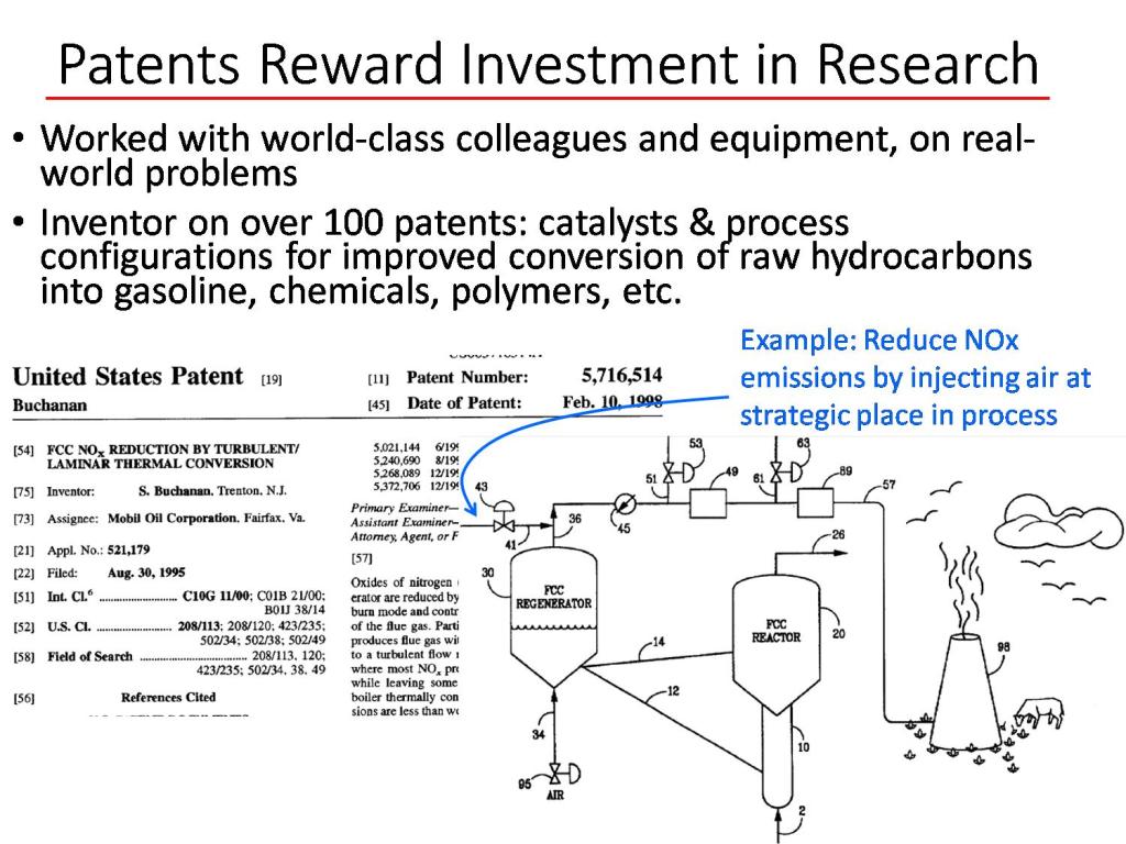
In my work in industrial research, I have been paid to develop technical improvements which could have economic value. A key incentive my company had for investing in this research was the expectation that if we came up with a novel improvement, that we could have exclusive rights to practice that improvement. There would have been little point in paying for research if our competitors could immediately make use of our hard-won insights. A snip of one of my patents is shown below.
For the world, and for most large groupings such as nations, the average income per capital is roughly equal to the average production per capita. The way to get more “stuff” (goods and services, and all their benefits) is to make more stuff. The way to make more stuff (per capita, and for fixed a workweek) is to make workers more productive. A key factor in productivity is technology. Two hundred years ago, nearly everyone in the U.S. had to be out in the sun and cold, working the soil, sowing by hand and plowing with the aid of animals, to grow enough food to feed everyone. Now I believe we are fed by only 2% of the workforce, using artificial fertilizers, improved seeds, huge tractors and combines, and satellite-aided computer scheduling. Most of the rest of us get to work in air-conditioned offices (or homes, in a pandemic year) and eat as much food as we want.
The patent system of the U.S. and other nations is designed to promote progress in productive technology. Early on, the newborn U.S. Congress passed the Patent Act of 1790, titled “An Act to promote the progress of useful Arts”. Without getting into all the legal details, a valid U.S. patent allows the inventor to exclude any other party from practicing their invention, for a period of twenty years. However, one of the requirement for a patent application is to clearly explain to the public how the invention works. When the twenty years is over, anyone can take advantage of the technology which the inventor has disclosed, which hopefully leads to widespread practice of technical improvements. While we can always ponder improvements to our system of patents, readers can thank it in part for many medical advances, and for delivering them from trudging behind a plow.
A balance sheet gives a snapshot of a corporation’s assets and liabilities. The difference between total assets and total liabilities is (by definition) the value of the equity owned by the owners or shareholders of the company.
With, say, a manufacturing firm, the assets would include tangible items such as buildings and equipment and inventory, and intangibles such as cash, bank accounts, and accounts receivable. Liabilities may include mortgages and other loans, and accounts payable such as taxes, wages, pensions, and bills for purchased goods.
The balance sheet for a bank is different. The “Assets” are mainly loans that the bank has made, plus some securities (such as US Treasury bonds) that the bank has purchased. These assets pay interest to the bank. The money the bank used to make these loans and purchase these securities came mainly from customer deposits or other borrowings by the bank (which are considered “Liabilities” of the bank), and also from paid-in capital from the bank owners/shareholders. [1] As usual, the current equity of the bank is assets minus liabilities. Thus:
The Federal Reserve System is a complex beast. We will not delve into all the components and moving parts, but just take a look at the overall balance sheet.
Unlike other banks, the Fed has the magical power of being able to create money out of thin air. Technically, what the Fed can do with that money is mainly make loans, i.e. buy interest-bearing securities such as government bonds. The Fed makes its transactions through affiliated banks, so it credits a bank’s reserve account with a million dollars, if it buys from that bank a million dollars’ worth of bonds. Those bonds then become part of the Fed’s “assets”, while the reserve account of the bank at the Fed (which is a liability of the Fed) becomes larger by a million dollars. Since the Fed is not a for-profit bank, the “Equity” entry on its balance sheet is nearly zero. Thus, total assets are essentially equal to total liabilities.
The Fed also has the power of literally printing money, in the form of Federal Reserve Notes (printed dollar bills). These, too, are classified as liabilities. Thus, you are probably carrying in your wallet right now some of the liabilities of the central bank of the United States.
Before 2008, the balance sheet of the Fed was under a trillion dollars. Nearly all the “Liabilities” were the Federal Reserve Notes and nearly all the “Assets” were US Treasury securities. The reserve accounts of the affiliated Depository Institutions was minuscule. All that changed with the Global Financial Crisis of 2008-2009. To help stabilize the financial system, the Fed started buying lots of various types of securities, including mortgage-backed securities (MBS) [2]. The Fed thus propped up the value of these securities, and injected cash (liquidity) into the system.
Here is a plot of how the assets of the Fed ballooned in the wake of the GFC, from about $ 0.9 trillion to over $ 4 trillion:
The initial purchases in 2008 were US Treasuries, which the Fed had prior authorization to do. To buy other securities, especially the mortgage products, required congressional authorization. The increased liabilities of the Fed which offset these purchases were mainly in the form of larger reserve accounts of the affiliated banks. The Fed started paying interest on these reserve accounts, to keep short term interest rates above zero at all times (otherwise the whole money market in the U.S. might implode).
With the Fed relentlessly buying the mortgage and bond products, the interest rates on long-term mortgages and bonds was kept low. This was deemed good for economic growth. The Fed tried to sell off some securities to taper down its balance sheet in 2018, but that effort blew up in its face – – the stock market started crashing in response in late 2018, and so the Fed backtracked . You can look at weekly tables of the Fed balance sheet here.
Anyway, the GFC and its aftermath provided the precedent for massive purchases of “stuff” by the Fed. When the Covid shutdown of the economy hit in March of this year, the Fed very quickly went into high gear. Its balance sheet shot up from $4 trillion to $7 trillion in just a few months. It bought not only Treasuries and MBS, but corporate bonds. This was way outside the Fed’s original charter, but the crisis was so intense that nobody seemed to care whether these actions were legal or not. And now, to finance the huge deficit spending of the federal government in the wake of the shutdowns, the Fed has been buying up nearly the entire issuance of Treasury bonds and notes.
These actions may have long term consequences we will explore in later posts [3]. For now, the Fed has made it clear that it will keep interests rates near zero for at least the next couple of years. Invest accordingly.
ENDNOTES
[1] Huge caveat: This statement gives the impression that a bank must first receive say a thousand dollar deposit before it can make a thousand dollar loan. That is not the case. The reality is just the opposite: the act of making a thousand dollar loan actually CREATES a corresponding thousand dollar deposit. This is very counterintuitive, and I won’t try to explain or justify this point here.
[2] Technically, the Fed is not “buying” the mortgage-backed security (MBS). Rather, it is making a “loan” to the bank, and holding the MBS as collateral against that loan.
[3] It is now harder to take the federal deficit seriously as a constraint on spending: the government can issue unlimited bonds to fund deficits, which the Fed will purchase to keep interest rates low. Yes, the government has to pay interest on those bonds, but the Fed has to return most of that interest to the Treasury, so the real cost to the government of that extra debt is low.
A week ago, we described commercial loans in general, and how they differ from bonds. Companies nearly always need money to make money, and thus have to borrow money in addition to selling stock shares. Companies that are new or smaller or doing poorly or have already borrowed a lot can still get loans, but these loans typically come with stringent conditions and require paying relatively high interest. These “leveraged loans” are the loan equivalent of “junk” bonds. When a bank lends money as a “Senior Secured Loan”, this entails agreements (“covenants”) which may specify that in event of default, this loan gets paid off ahead of any other creditor, and also that some specific asset held by the company, such as a building or an oil field, will be given over to the bank.
Financial institutions like insurance companies and pension funds are hungry for “investment grade” securities like bonds rated BBB or higher. Normally, these institutions would not consider buying into the senior loan marketplace, since these instruments are not considered investment grade.
Enter “Collateralized Loan Obligations” (CLOs). With a CLO, 200 or so loans which have been made by banks and then sold off into the market are bundled together, and then the cash flow from the interest paid on these loans plus the principal paid back is repackaged into slices or “tranches”. The highest level tranches get first dibs on being paid from the overall CLO cash flow, then the lower and lower tranches. The majority of bank loans today end up being packaged into CLOs. CLOs are an example of a lucrative operation known as “securitization”: “Securitization is the process of taking an illiquid asset or group of assets and, through financial engineering, transforming it (or them) into a security” (per Investopedia).
The rate of loan defaults in recent years has been only 3-4%, and on average the recovery on a given defaulted senior secured loan has been around 80%. So the actual losses (e.g. 4% x 20%, or 0.8% net) have been quite low. The highest annual default rate in recent memory was about 10%, in the Global Financial Crisis of 2008-2009.
The theory is that, although any particular loan has a nontrivial chance of defaulting, it is unthinkable that more than say 20% of all loans would default; and even if a full 20% of the loans did default, we would expect that the actual losses after liquidating the pledged collateral would be more like 4% of the entire loan portfolio (i.e. 20% defaults x 20% loss per default). This means that the top 95% or so of CLO cash flow should be considered very secure, and the top 60-70% are utterly secure.
Thus, the top 60-65% of the CLO cash flow is packaged as super secure, relatively low-yielding AAA rated debt, and as such is bought up by conservative financial institutions, including banks. This arrangement keeps those institutions happy, and also facilitates the making of loans to the needy companies who are taking out the underlying loans.
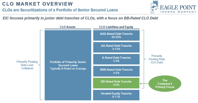
The figure below from an Eagle Point Investment Company presentation depicts typical CLO tranches:
The lower the position in the CLO cash flow “waterfall”, the higher the yield and the higher the risk of non-payment. The AA, A, and BBB debt tranches are all considered investment grade, though with higher risk and higher yields than the AAA tranche. The Eagle Point Investment Company happens to buy into the BB-rated debt tranche, which is just below investment grade. You, the public, can buy shares Eagle Point Investment (stock symbol EIC). These shares pay about 7% yield, after hefty management fees have been subtracted.
The equity tranche lies at the very bottom of the CLO heap. If there were, say, 20% loan defaults with only 50% recovery of the loans, the equity tranche might get completely wiped out. So these are more risky investments. As usual, there is high reward along with the risk. Oxford Lane Capital (OXLC) deals in CLO equity, and it will pay you about 15% per year, which is huge in today’s low-interest world. But….you need to be prepared to have the stock value cut in half every ten years or so, whenever there is a big hiccup in the financial world.
Anyone who was an economics-savvy adult during the GFC should be asking, “But, but, but…aren’t these CLOs essentially the same thing as the collateralized debt obligations (CDOs) that blew up the world in 2008?” The answer is partly yes, in that in both cases a bunch of loans get bundled together and then resliced into tranches. That said, we hope that the underlying loans in today’s CLOs are more robust than the massively shady home mortgage loans of 2003-2008 that fed into those CDOs. Back then, unscrupulous banks and mortgage companies handed out thousands of housing loans to ill-informed private individuals who did not remotely qualify for them, and then the banks dumped these loans out into the broader financial markets via CDOs. The bank loans behind today’s CLOs are more sober, serious, vetted affairs than those ridiculous subprime home mortgages.
This past summer, in the thick of the Covid shutdowns which have stressed small businesses, The Atlantic published a dire assessment of the potential for CLOs to sink the system, with the catchy title The Looming Banks Collapse . The article noted, fairly enough, that there has been a trend in the past few years to weaken the covenants on loans which would normally protect the lender against losses. Most loans these days are considered “covenant-lite”, compared to several years ago. There is genuine concern that the recovery on these loans might be more like 40-50%, instead of the historic 70-80%. On the other hand, the looser requirements on these loans may mean that fewer of them will technically violate these looser covenants and thus fewer companies will actually default. A recent survey estimates that the default rate in the $ 1.2 trillion dollar leveraged loan universe will peak at only 6.6% in 2021.
Also, today’s CLOs seem to be rated by the major ratings agencies more responsibly than the notoriously optimistic ratings given to CDO’s back in 2008. “CLOs are usually rated by two of the three major ratings agencies and impose a series of covenant tests on collateral managers, including minimum rating, industry diversification, and maximum default basket”, according to an article by S&P Global Market Intelligence. That article has a good description of CLOs, including a brief tutorial video on the nuts and bolts of how they work.
My dear friend Mark Lutter has had me all riled up about charter cities for a few years now. I link to a new podcast from USFQ’s Aula Magna magazine on the subject that gives a very short introduction to the topic. After recording the podcast I returned to preping a class on genetic algorithms and got all riled up because I saw a connection between the two I hadn’t seen (clearly) before. Charter cities can be real life genetic algorithms for institutional innnovation.
Genetic algorithms are a form of machine learning that searches for solutions to problems by trying out a variety of solutions. As the name implies they are based on the evolutionary algorithm of diversity-selection-amplification to adapt solutions. In a genetic algorithm a population of of possible solutions to an optimization problem is instantiated and solutions with high fitness and reproduce (using cross over, mutation, and other genetic operators) to create new populations of solutions. over enough iterations genetic algorithms are goods ways to search for solutions whe the solution space is complex and poorly defined, which is probably what institutional space looks like.
Now imagine a country that is designed as a genetic algorithm and charter cities within the country as posible institutional solutions. The constitution of the central government is the overall framework of the genetic algorithm and the diversity of institutional arrangments at local government levels (i.e. different charters) are posible solutions.
Viewing charter cities in this light, the interesting question now turns to the rules of the central government and not necesarily to the rules implemented by the charters themselves.
A few of the questions that have begun to bother me follow. What country level rules lead to convergence, or at least continual adaptation to better institutional arrangments at the local level? What should the constriants be imposed on the charters for better, faster convergence and learning? Zoning and housing restrictions would be a clear impediment to convergence as they limit foot voting. If we view charter cities (and fiscal federalism) as an experiment to search for solutions to institutional arrangements for governance, can we use the criteria used by IRB boards as the minimum set of requirements that informa the central government constitution/framework where this experiment takes place?
Continuing on the theme of last week’s minimum wage increase in Florida, there are two interesting papers recently accepted for publication that both cover the 1966 Fair Labor Standards Act. This law extended the federal minimum wage to a number of previously uncovered. Crucially, the newly covered industries employed a large number of African-American workers.
The two papers agree on some points, such as that African Americans saw large wage gains following the increase. But was there a disemployment effect? Here is where the papers differ.
Ellora Derenoncourt and Claire Montialoux’s paper “Minimum Wages and Racial Inequality” is forthcoming in the Quarterly Journal of Economics. Here is what they find: “We can rule out significant disemployment effects for black workers. Using a bunching design, we find no aggregate effect of the reform on employment.”
So who is right? Let me clearly state here that both of these papers are very well done, both in their methods and in their assembling of historical data. But I think there is a key difference in the samples they analyze: Derenoncourt and Montialoux’s paper only includes workers aged 25-55. Bailey and co-authors use a broader age range, 16-64, which importantly includes teenagers (this is discussed in Section D of their online appendix).
Since teenagers and other young workers are the ones we suspect are going to be most impacted by the minimum wage (much of the literature focuses on teenagers), the exclusion of workers under 25 seems like a curious omission, and a reason I tempted to believe the results of Bailey and co-authors. But Derenoncourt and Montialoux do try to justify their choice of age group: 1. workers under 21 were subject to a different minimum wage; and 2. workers under 25 were subject to the draft for the Vietnam War.
So once again, you might ask, who is right? I will admit here that I don’t know. Standard economic theory suggests that disemployment effects will result from a legal minimum wage (I fully acknowledge the emerging literature on monopsony power, but I maintain this is still not the standard analysis), and especially so for teenagers and young workers. So I am skeptical of any analysis which excludes these workers, whatever other merits it may have.
Here’s my take: we probably can’t tell much about how the minimum wage will impact young workers today based on these studies. If Derenoncourt and Montialoux’s reasons for removing young workers are indeed sound, then we aren’t really testing the question most economists are interested in today (so I would caution against their attempt to apply the results to labor markets today). But that doesn’t mean these aren’t interesting papers to read on an important change in the history of minimum wage laws in the US!