The NSCH is the latest casualty of the new administration taking down major datasets from government websites. Between Archive.org and what I had downloaded for old projects, I was able to get all the 2016-2023 topical NSCH files and post them on an Open Science Foundation page.
I took this as a chance to improve the data- the government previously only made the topical Public Use Files available in SAS and Stata formats one year at a time, so I added a merged version for all available years in both Stata and Excel formats.
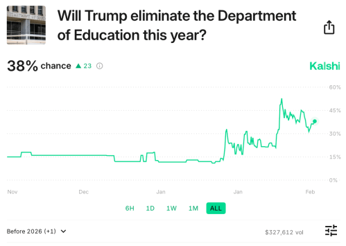
I hope and expect that the National Survey Children’s Health will be back up at official websites soon. But I expect that other datasets will be taken down permanently, so now is the time to download what you think you might need and add it to your data hoard– especially if you want anything from the Department of Education.
That post was partly inspired by critics of the unemployment rate as a broad measure of labor market utilization. Yes, the UR isn’t perfect, and it misses some things. But other measures of labor force performance tend to move with the UR, and so it’s still a useful measure. 2023 saw not only some of the lowest unemployment rates in US history (rivaling the late 1960s), but also some of the highest employment rates (only beat by the late 1990s). Wage growth was also robust. And other measures of unemployment, such as the much broader U-6 rate and the Insured Unemployment Rate, were also at record low levels (though the data doesn’t go back as far).
Today I learned about a very interesting, though I think probably confusing, measure called the “true unemployment rate.” Produced by the Ludwig Institute, it uses the same underlying data source (the CPS) that the BLS uses to calculate the unemployment rate and other measures mentioned above. This “true” rate is definitely intended to shock you: it suggests that 25 percent of the workforce is “unemployed.”
But they aren’t actually measuring unemployment. What they are doing, in a sense, is combining a very broad measure of labor underutilization (like the U-6 rate mentioned above) with a measure that is similar to the poverty rate (but not exactly). They count people as unemployed if they are part-time workers, but would like to work full-time (U-6 does this). But they also count you as unemployed if you earn under $25,000 per year. Or if you don’t work at all, you are counted as unemployed — even if you aren’t trying to find a job (such as being a student, a homemaker, disabled, etc.). The entire working age population (ages 16+, though they don’t tell us the upper limit, we can probably assume 64) is the denominator in this calculation.
So again, this is attempting to combine a broad measure of employment with a poverty measure (though here poverty is defined by your own wage, rather than your household income). So of course you will get a bigger number than the official unemployment rate (or even the U-6 rate).
But here’s the thing: even with this much broader definition, the US labor market was still at record lows in 2023! Given this new information I learned, and that we are now through 2024, I decided to update the table from my previous post:
From this updated table, we see that by almost every measure, 2023 was an excellent year for the US labor market. The only measure where it slightly lags is the prime-age employment rate, which was a bit higher in the late 1990s/2000. Real wage growth was also quite strong in 2023, despite still having some lingering high inflation from the 2021-22 surge.
How about 2024? By almost all of these measures, 2024 was slightly worse than 2023. And still, 2024 was a good year. A pretty, pretty good year for the labor market. And while the UR ticked up in the middle of the year, it has since come back down a bit and is now right at 4%. As for the “true” unemployment rate, it followed a similar pattern, ticking up a bit in mid-2024, but by December it was back slightly below the level from December 2023.
Alternative “true” measures of the economy rarely give us any additional information than the standard measures — other than a shocking, but confusing, headline number.
Like many Principles of Macroeconomics courses, mine begins with an introduction to GDP. We motivate RGDP as a measure of economic activity and NGDP as an indicator of income or total expenditures. But how does more RGDP imply that we are better off, even materially? One entirely appropriate answer is that the quantities of output are greater. Given some population, greater output means more final goods and services per person. So, our real income increases. But what else can we say?
First, after adjusting for price changes, we can say that GDP underestimates the value that people place on goods and services that are transacted in markets. Given that 1) demand slopes down and 2) transactions are consensual, it stands to reason that everyone pays no more than their maximum value for things. This implies that people’s willingness to pay for goods surpasses their actual expenditures. Therefore, RGDP is a lower bound to the economic benefits that people enjoy. Without knowing the marginal value that people place on all quantities less than those that they actually buy, we have no idea how much more value is actually provided in our economy.
Several major datasets produced by the federal government went offline this week. Some, like the Behavioral Risk Factor Surveillance Survey and the American Community Survey, are now back online; probably most others will soon join them. But some datasets that the current administration considers too DEI-inflected could stay down indefinitely.
This serves as a reminder of the value of redundancy- keeping datasets on multiple sites as well as in local storage. Because you never really know when one site will go down- whether due to ideological changes, mistakes, natural disasters, or key personnelmoving on.
If you are currently looking for a federal dataset that got taken down, some good places to check are IPUMS, NBER, Archive.org, or my data page. PolicyMap has posted some of the federal datasets that seem particularly likely to stay down; if you know of other pages hosting federal datasets that have been taken down, please share them in the comments.
Donald Trump has repeatedly said that the US was at our “richest” or “wealthiest” in the high-tariff period from 1870-1913, and sometimes he says more specifically in the 1890s. Is this true?
One possibility is tax revenue, since he often says this in the context of tariffs versus an income tax. Broadly this also can’t be true, as federal revenue was just about 3% of GDP in the 1890s, but is around 16% in recent years.
But perhaps it is true in a narrower sense, if we look at taxes collected relative to the country’s spending needs. Trump has referenced the “Great Tariff Debate of 1888” which he summarized as “the debate was: We didn’t know what to do with all of the money we were making. We were so rich.” Indeed, this characterization is not completely wrong. As economic historian and trade expert Doug Irwin has summarized the debate: “The two main political parties agreed that a significant reduction of the budget surplus was an urgent priority. The Republicans and the Democrats also agreed that a large expansion in government expenditures was undesirable.” The difference was just over how to reduce surpluses: do we lower or raise tariffs?
It does seem that in Trump’s mind being “rich” in this period was about budget surpluses. Let’s look at the data (I have truncated the y-axis so you can actually read it without the WW1 deficits distorting the picture, but they were huge: over 200% of revenues!):
It is certainly true that under parts of the high-tariff period, we did collect a lot of revenue from tariffs! In some years, federal surpluses were over 1% of GDP and 30% of revenues collected. But notice that this is not true during Trump’s favored decade, the 1890s. Following the McKinley Tariff of 1890, tariff revenue fell sharply (though probably not likely due to the tariff rates, but due to moving items like sugar to the duty-free list, as Irwin points out). The 1890s were not a decade of being “rich” with tariff revenue and surpluses.
Finally, also notice that during the 1920s the US once again had large budget surpluses. The income tax was still fairly new in the 1920s, but it raised around 40-50% of federal revenue during that decade. By the Trump standard, we (the US federal government) were once again “rich” in the 1920s — this is true even after the tax cuts of the 1920s, which eventually reduced the top rate to 25% from the high of 73% during WW1.
If we define a country as being “rich” when it runs large budget surpluses, the US was indeed rich by this standard in the 1870s and 1880s (though not the 1890s). But it was rich again by this standard in the 1920s. This is just a function of government revenue growing faster than government spending. And the growth of revenue during the 1870s and 1880s was largely driven by a rise in internal revenue — specifically, excise taxes on alcohol and tobacco (these taxes largely didn’t exist before the Civil War).
1890 was the last year of big surpluses in the nineteenth century, and in that year the federal government spent $318 million. Tariff revenue (customs) was just $230 million. There was only a surplus in that year because the federal government also collected $108 million of alcohol excise taxes and $34 million of tobacco excise taxes. In fact, throughout the period 1870-1899, tariff revenues are never enough to cover all of federal spending, though they do hit 80% in a few years (source: Historical Statistics of the US, Tables Ea584-587, Ea588-593, and Ea594-608):
One more thing: in some of these speeches, Trump blames the Great Depression on the switch from tariffs to income taxes. In addition to there really being no theory for why this would be the case, it just doesn’t line up with the facts. The 1890s were plagued by financial crises and recessions. The 1920s (the first decade of experience with the income tax) was a period of growth (a few short downturns) and as we saw above, large budget surpluses. The Great Depression had other causes.
Most of us know about FRED, the Federal Reserve Economic Data hosted by the Federal Reserve of St. Louis. It provides data and graphs at your fingertips. You can quickly grab a graph for a report or for a online argument. Of course, you can learn from it too. I’ve talked in the past about the Excel and Stata plugins.
But you may not know about the FRED FRASER. From their about page, “FRASER is a digital library of U.S. economic, financial, and banking history—particularly the history of the Federal Reserve System”. It’s a treasure trove of documents. Just as with any library, you’re not meant to read it all. But you can read some of it.
I can’t tell you how many times I’ve read a news story and lamented the lack of citations – linked or unlinked. Some journalists seem to do a google search or reddit dive and then summarize their journey. That’s sometimes helpful, but it often provides only surface level content and includes errors – much like AI. The better journalists at least talk to an expert. That is better, but authorities often repeat 2nd hand false claims too. Or, because no one has read the source material, they couch their language in unfalsifiable imprecision that merely implies a false claim.
A topical example would be the oft repeated blanket Trump-tariffs. That part is not up for dispute. Trump has been very clear about his desire for more and broader tariffs. Rather, economic news often refers back to the Smoot-Hawley tariffs of 1930 as an example of tariffs running amuck. While it is true that the 1930 tariffs applied to many items, they weren’t exactly a historical version of what Trump is currently proposing (though those details tend to change).
How do I know? Well, I looked. If you visit FRASER and search for “Smoot-Hawley”, then the tariff of 1930 is the first search result. It’s a congressional document, so it’s not an exciting read. But, you can see with your own eyes the diversity of duties that were placed on various imported goods. Since we often use the example of imported steel and since the foreign acquisition of US Steel was denied, let’s look at metals on page 20 of the 1930 act. But before we do, notice that we can link to particular pages of legislation and reports – nice! Reading the Smoot-Hawley Tariff Act’s original language, we can see the diverse duties on various metals. Here are a few:
The US Equal Opportunity Commission identifies characteristics by which an employee can’t be harassed, hired, paid, or promoted. A challenge with enforcing the non-discriminatory standards is that the evidence must be a slam dunk. There needs to be a smoking gun of a paper trail, recorded conversation, or multiple witnesses. Mere statistical regularities are insufficient for demonstrating that characteristics like race, age, or sex are being considered inappropriately.
If employees are all identically qualified, then we’d expect the employment at a firm to reflect the characteristics of the applicant pool, within a margin of error due to randomness. One difficulty is that plenty of discrimination can occur within that margin of error. A firm may not have sexist policies, but a single manager can be sexist once or even multiple times and still keep the firm-level proportions within the margin of error. This is especially stark if the company managers or officers are the primary positions for which discrimination occurs.
Another difficulty is that randomness can cause extreme proportions of employee characteristics. Having a workplace that is 95% male when the applicant pool is 60% male isn’t necessarily discriminatory. In fact, given a sample size, we can calculate how likely such an employee distribution would occur by randomness. Even by randomness, extreme proportions will inevitably occur. As a result, lawsuits or complaints that have only statistical evidence of this sort don’t go very far and tend not to win big settlements.
But this doesn’t stop firms from avoiding the legal costs anyway. Firms generally prefer not to have regulatory authorities snooping around and investigating. Most people break some laws even unintentionally or innocuously, and a government official on the premises increases the expected compliance costs. Further, even if untrue accusations are made, legal costs can be substantial. Therefore, firms have an incentive to ensure that they can somehow demonstrate that they are not being discriminatory based on legally protected characteristics.
However, as I said, extreme proportions happen randomly. If those extremes are interpreted as evidence of illegal discrimination, then the firms have an incentive to hire among identical applicants in a non-random manner. They have an incentive to tilt the scales of who gets hired in favor of achieving a specific distribution of race, sex, etc. People have a variety of feelings about this. Some call it ‘reverse discrimination’ or discrimination against a group that has not historically experienced widespread disfavor. Others say that hiring intentionally on protected characteristics can help balance the negative effects of discrimination elsewhere. I’m not getting into that fight.
The average price of a dozen eggs is back up over $4, about the same as it was 2 years ago during the last avian flu outbreak. Egg prices are up 65% in the past year. But does that mean the grocery inflation we experienced in 2021-22 is roaring back?
No really. Spending on eggs is around 0.1% of all consumer spending, and just about 2% of consumer spending on groceries. Symbolically, it may be important, since consumers pick up a dozen eggs on most shopping trips. But to know what’s going on with groceries overall, we have to look at the other 98% of grocery spending.
It’s been a wild 4 years for grocery prices in the US. In the first two years of the Biden administration, grocery prices soared over 19%. But in the second two years, they are up just 3% — pretty close to the decade average before the pandemic (even including a few years with grocery deflation!).
As any consumer will tell you, just because the rate of inflation has fallen doesn’t mean prices on average have fallen. Prices are almost universally higher than 4 years ago, but you can find plenty of grocery items that are cheaper (in nominal terms!) than 1 or 2 years ago: spaghetti, white bread, cookies, pork chops, chicken legs, milk, cheddar cheese, bananas, and strawberries, just to name a few (using BLS average price data).
There is no way to know the future trajectory of grocery prices, and we have certainly seen recent periods with large spikes in prices: in addition to 2021-22, the US had high grocery inflation in 2007-2009, 1988-1990, and almost all of the period from 1972-1982 (two-year grocery inflation was 37% in 1973-74!). Undoubtedly grocery prices will rise again. But the welcome long-run trend is that wages, on average, have increased much faster than grocery prices:
Don’t worry, EWED is in the same place as always, but my personal website is moving.
Temple University has generously hosted my site long after my 2014 graduation. But next week they are moving to a more typical policy where alumni lose access to online university resources like web-hosting, email, and library datasets starting one year after graduation.