Iso-Standard Error & Economist Unemployment

Say that I want to calculate the unemployment rate by college major. That’s easy enough – we just divide the number of unemployed people by the number of people who are in the labor force. Repeat for each major.  The 2024 ACS includes all the variables we need, including employment status by week, but here I just calculate the annual average. I’ll calculate unemployment rates using the unweighted observations because I want to make a separate statistical point about simple standard errors.

Sample weights aside, we have some basic data maintenance to consider. The sample sizes for each major differ. Some majors include more than 15k people, while others have less than 100. Which majors should I include? All of them?

It depends on how precise I want the estimates to be – how small I want the standard errors to be. Below is the basic equation for the standard error (SE). Maybe I want my standard errors to be no more than 0.1%, since unemployment rates are on the order of 1-5%*. Then, it’s just a simple matter of setting the SE equation equal to 0.001 and solving…. Except that there are two variables. Getting a SE of 0.1% depends on both the sample size and the observed proportion. So, a basic rule such as ‘include only majors with at least 100 people won’t quite achieve what we want since the whole point of the exercise is that we suspect that the proportions of unemployed people differ among majors.

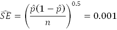
In order to get an idea of how many observations we need conditional on the proportion, we can use a popular tool in economics. Basically, adding the prefix “iso” to any term lets us see how two (or more!) other variables matter for the value of the term. We have iso-costs, iso-quants, iso-Sharpes, iso-retirement payments, etc. Here, we can have an iso-standard error by graphing the sample size on one axis, and the proportion on the other. With the desired SE as a constant, we can rearrange the SE equation so that  the sample size and proportion variables remain. They’re isolated below – solving for sample size is much simpler.  

The above equations let us see all of the sample size and proportion combinations that yield an arbitrary standard error. We’re basically doing the first steps of what’s known as a power calculation. We’re setting up some guard rails before doing the analysis so that we know ahead of time whether we’d even be able to tell the difference between proportions with the sample sizes that we have. Below is the graph of the iso-SE to illustrate the sample size & proportion combinations that yield some target SEs. Pictured is the left side of parabolas. What does it tell us? It tells us that shrinking the target SE increases the necessary sample size at each proportion REALLY FAST.

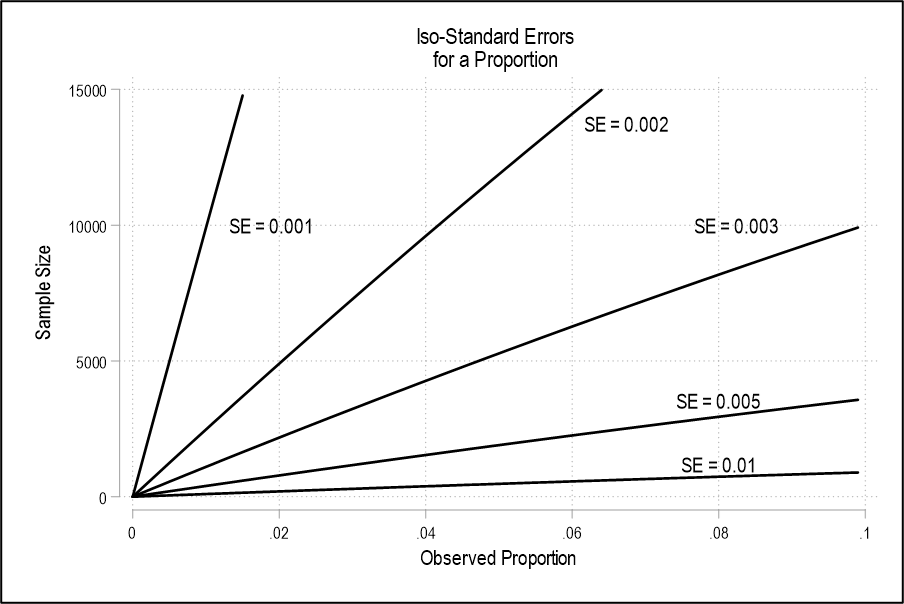
Since the most college majors have a sample size that is well below 15k, we basically know ahead of time that we won’t be able to tell the difference between their unemployment rates if they differ by a mere tenth of a percent. Given that the national unemployment rate in 2024 was around 4% and around 2.3% for college majors, there’s not much room for error – literally. Everything looks the same when proportions are similar and sample sizes are small.

Continue reading →