Writing with ChatGPT Buchanan Seminar on YouTube

I was pleased to be a (virtual) guest speaker for Plateau State University in Nigeria. My host was (Emergent Ventures winner) Nnaemeka Emmanuel Nnadi. The talk is up on Youtube with the following timestamp breakdown:

During the first ten minutes of the video, Ashen Ruth Musa gives an overview called “The Bace People: Location, Culture, Tourist Attraction.”

Then I introduce LLMs and my topic.

Minute 19:00 – 29:00 is a presentation of the paper “ChatGPT Hallucinates Nonexistent Citations: Evidence from Economics“

Minute 23:30 – 34 is summary of my paper “Do People Trust Humans More Than ChatGPT?”

Continue reading →

Forecasting Swing States with Economic Data

Ray Fair at Yale runs one of the oldest models to use economic data to predict US election results. It predicts vote shares for President and the US House as a function of real GDP growth during the election year, inflation over the incumbent president’s term, and the number of quarters with rapid real GDP growth (over 3.2%) during the president’s term.

Currently his model predicts a 49.28 Democratic share of the two-party vote for President, and a 47.26 Democratic share for the House. This will change once Q3 GDP results are released on October 30th, probably with a slight bump for the dems since Q3 GDP growth is predicted to be 2.5%, but these should be close to the final prediction. Will it be correct?

Probably not; it has been directionally wrong several times, most recently over-estimating Trump’s vote share by 3.4% in 2020. But is there a better economic model? Perhaps we should consider other economic variables (Nate Silver had a good piece on this back in 2011), or weight these variables differently. Its hard to say given the small sample of US national elections we have to work with and the potential for over-fitting models.

But one obvious improvement to me is to change what we are trying to estimate. Presidential elections in the US aren’t determined by the national vote share, but by the electoral college. Why not model the vote share in swing states instead?

Doing this well would make for a good political science or economics paper. I’m not going to do a full workup just for a blog post, but I will note that the Bureau of Economic Analysis just released the last state GDP numbers that they will prior to the election:
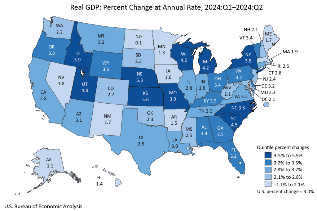
Mostly this strikes me as a good map for Harris, with every swing state except Nevada seeing GDP growth above the national average of 3.0%. Of course, this is just the most recent quarter; older data matters too. Here’s real GDP growth over the past year (not per capita, since that is harder to get, though it likely matters more):

RegionReal GDP Growth Q2 2023 – Q2 2024
US3.0%
Arizona2.6%
Georgia3.5%
Michigan2.0%
Nevada3.4%
North Carolina4.4%
Pennsylvania2.5%
Wisconsin3.3%

Still a better map for Harris, though closer this time, with 4 of 7 swing states showing growth above the national average. I say this assuming as Fair does that the candidate from the incumbent President’s party is the one that will get the credit/blame for economic conditions. But for states I think it is an open question to what extent people assign credit/blame to the incumbent Governor’s party as opposed to the President. Georgia and Nevada currently have Republican governors.

Overall I see this as one more set of indicators that showing an election that is very close, but slightly favoring Harris. Just like prediction markets (Harris currently at a 50% chance on Polymarket, 55% on PredictIt) and forecasts based mainly on polls (Nate Silver at 55%, Split Ticket at 56%, The Economist / Andrew Gelman at 60%). Some of these forecasts also include national economic data:
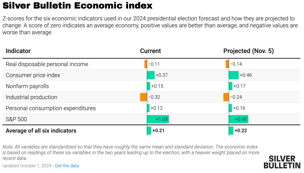
Gelman suggests that the economy won’t matter much this time:

We found that these economic metrics only seemed to affect voter behaviour when incumbents were running for re-election, suggesting that term-limited presidents do not bequeath their economic legacies to their parties’ heirs apparent. Moreover, the magnitude of this effect has shrunk in recent years because the electorate has become more polarised, meaning that there are fewer “swing voters” whose decisions are influenced by economic conditions.

But while the economy is only one factor, I do think it still matters, and that forecasters have been underrating state economic data, especially given that in two of the last 6 Presidential elections the electoral college winner lost the national popular vote. I look forward to seeing more serious research on this topic.
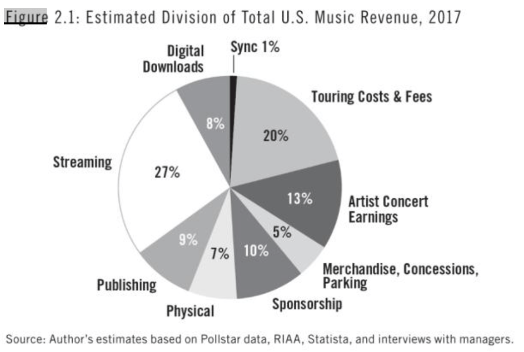
Rockonomics Highlights

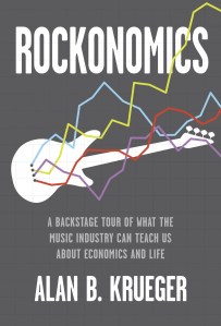
I missed Alan Kreuger’s 2019 book on the economics of popular music when it first came out, but picked it up recently when preparing for a talk on Taylor Swift. It turns out to be a well-written mix of economic theory, data, and interviews with well-known musicians, by an author who clearly loves music. Some highlights:

[Music] is a surprisingly small industry, one that would go nearly unnoticed if music were not special in other respects…. less than $1 of every $1,000 in the U.S. economy is spent on music…. musicians represented only 0.13 percent of all employees [in 2016]; musicians’ share of the workforce has hovered around that same level since 1970.

there has been essentially no change in the two-to-one ratio of male to female musicians since the 1970s

The gig economy started with music…. musicians are almost five times more likely to report that they are self-employed than non-musicians

30 percent of musicians currently work for a religious organization as their main gig. There are a lot of church choirs and organists. A great many singers got their start performing in church, including Aretha Franklin, Whitney Houston, John Legend, Katy Perry, Faith Hill, Justin Timberlake, Janelle Monae, Usher, and many others

Continue reading →

Paper on Finance and Economics Women Club

I am one of several founders of a club with the abbreviation F.E.W. for Finance and Economics Women. This is a student organization that we have at Samford and that Dr. Darwyyn Deyo runs at San Jose State University.

Read our report here: The Finance and Economics Women’s Network (FEW): Encouraging and Engaging Women in Undergraduate Programs published in the Journal of Economics and Finance Education

Our short paper is mostly a how-to guide including a draft of a club charter document. We describe our institutions and how we use this group to engage and encourage students. Please read it for more details on how to start a club.

Like most student groups, the FEW model relies on student leaders who take initiative. Having done this for more than 6 years, we have a growing network of alumni and local business partners who connect to current students through FEW events. Personally, I am lucky that 3 faculty members total support the club at my school.

Women are often minorities in upper-division econ and finance classes. Women also have some unique challenges when it comes to choosing career paths and navigating the workplace. These events (e.g. bringing in a manager from a local bank to talk with student over lunch) allow a space for students to ask questions they might not normally ask in a classroom setting or in a standard networking environment.

We report the results of a small survey in our paper. We can’t infer causality, nor did we run any experiments. However, we did find that women were more likely to report that a role model in their chosen profession influenced their choice of major. Part of the purpose of the FEW model is to expose students to a variety of role models who they might not otherwise connect with.

Here’s a news article with a picture of the founding group at Samford. I have great appreciation and respect for our student leaders who keep it going, and I am grateful to the graduates who stay in contact with us.

Suggested citation: Buchanan, Joy, and Darwyyn Deyo, “Finance and Economics Women’s (FEW) Network: Encouraging and Engaging Women in Undergraduate Programs” (2023) Journal of Economic and Finance Education, 22: 1, 1-14.

Interpreting New DIDs

If you didn’t know already, the past five years has been a whirl-wind of new methods in the staggered Differences-in-differences (DID) literature – a popular method to try to tease out causal effects statistically. This post restates practical advice from Jonathan Roth.

The prior standard was to use Two-Way-Fixed-Effects (TWFE). This controlled for a lot of unobserved variation over individuals or groups and time. The fancier TWFE methods were interacted with the time relative to treatment. That allowed event studies and dynamic effects.

Continue reading →

The Economics of Taylor Swift

Cowen’s 2nd Law states that there is a literature on everything. I would certainly expect there to be a literature on the best-selling musician in the world. And of course there is; Google Scholar returns 23,500 results for “Taylor Swift”, and we’ve done 5 posts here at EWED. But surprisingly, searching EconLit returns nothing, suggesting there are currently no published economics papers on Taylor Swift, though searching “Taylor” and “Swift” separately reveals hundreds of articles about the Taylor Rule and the SWIFT payment system. Google Scholar does report some economics working papers about her, but the opportunity to be the first to publish on Taylor Swift in an economics journal (and likely get many media interview requests as a result) is still out there.

Swift presents a variety of angles that could be worthy of a paper; re-recording her masters forcopyright reasons, her efforts to channel concert tickets to loyal fans over re-sellers, or her sheer macroeconomic impact. I’ve added a note about this to my ideas page (where I share many other paper ideas).

In the mean time, I’ll be giving a short talk on the Economics of Taylor Swift at 7pm Eastern on Monday, September 16th, as part of a larger online panel. The event is aimed at Providence College alumni, but I believe anyone can register here.

Update 10/25/24: A recording of the event is here, and a recording of a followup interview I did with local TV is here.

Leave Me Alone and I’ll Make You Rich

That is the title of a 2020 book by Dierdre McCloskey and Art Carden. It attempts to sum up McCloskey’s trilogy of huge books on the “Bourgeois Virtues” in one short, relatively easy to read book. I haven’t read the full trilogy, so I can’t say how good the new book is as a distillation, but I found that it was easy to read and at least makes me think I understand McCloskey’s basic thesis for why the world got rich. I share some highlights here.

Part 1 of the book aims to establish that the world did in fact get richer over recent centuries, plus give a basic explanation of liberal political thought. If you already know this you could skip this part and cut down an easy 189 page read to a very easy 106 page read (part 1 is for some reason written in a way that assumes you disagree with the authors, which grates when you don’t, or perhaps also if you do).

Part 2 gets to what I at least came for- digging into the history to solve the puzzle of why the Industrial Revolution / Great Enrichment took off when and where it did. Which means first, explaining why many things people think made 18th century England special were actually common elsewhere, like markets:

Continue reading →

Sticky Prices as Coordination Failure Working Paper

“Sticky Prices as Coordination Failure: An Experimental Investigation” is my new paper with David Munro of Middlebury, up at SSRN.

We ask whether coordination failures are a source of nominal rigidities. This was suggested in a recent speech by ECB President Christine Lagarde. She said, “In the recent decades of low inflation, firms that faced relative price increases often feared to raise prices and lose market share. But this changed during the pandemic as firms faced large, common shocks, which acted as an implicit coordination mechanism vis-à-vis their competitors.”

Coordination failure was suggested as a possible cause of price rigidity in a theory paper by Ball and Romer (1991). They demonstrated the possibility for multiple equilibria, and we perform the first laboratory test to observe equilibrium selection in this environment.

We theoretically solve a monopolistically competitive pricing game and show that a range of multiple equilibria emerges when there are price adjustment costs (menu costs). We explore equilibrium selection in laboratory price setting games with two treatments: one without menu costs where price adjustment is always an equilibrium, and one with menu costs where both rigidity and flexibility are possible equilibria.

In plain language, for our general audience, the idea is that the prices you set might depend on what other people are doing. If other people are responding to a shock (for example, Covid driving up labor costs all over town might cause retail prices to rise) then you will, too. If every other store in town is afraid to raise prices, then there is a certain situation where you might resist adjusting your prices, too (price rigidity).

Results: First, when there is only one theoretical equilibrium, subjects usually conform to it. When cost shocks are large, price adjustment is a unique equilibrium regardless of the presence of menu costs, and we see that subjects almost always adjust prices. When cost shocks are small and there are menu costs rigidity is a unique equilibrium and subjects almost never adjust. Conversely, with small cost shocks subjects almost always adjust when there are no menu costs.

The more interesting cases are when the parameters allow for either rigidity or flexibility to be selected. We find that groups do not settle at the rigidity equilibrium. Rather, depending on the specific nature of the shock, between half and 80% of subjects adjust in response to a shock. The intermediate levels of adjustment are represented here in this figure as the red circles that fall between the red and green bands where multiple equilibria are possible.

In the figure above, the red circles are higher when the production cost shock gets further from zero in absolute value. We see that the proportion of subjects adjusting prices is proportional to the size of the cost shocks. This is consistent with the interpretation that the large post-COVID cost shocks acted as an implicit coordination mechanism for firms raising prices. Our results provide a number of interesting insights on nominal rigidities. We document more nuance in the paper regarding heterogeneity and asymmetry. Comments and feedback are appreciated! If it’s not clear from the EWED blog how to email me (Joy), find my professional contact info here. 

A Continually Updated Bernanke-Taylor Rule

Despite its many flaws*, I always like to check in on what the Taylor Rule suggests for the Fed. Its virtues are that it gives a definite precise answer, and that it has been agreed upon ahead of time by a variety of economists as giving a decent answer for what the Fed should do. Without something like the Taylor Rule, everyone tends to grasp for reasons that This Time Is Different. Academics seek novelty, so would rather come up with some new complex new theory of what to do instead of something undergrads have been taught for years. Finance types tend to push whatever would benefit them in the short term, which is typically rate cuts. Political types push whatever benefits their party; typically rate cuts if they are in power and hikes if not, though often those in power simply want to emphasize good economic news while those out of power emphasize the bad news.

The Taylor Rule can cut through all this by considering the same factors every time, regardless of whether it makes you look clever, helps your party, or helps your returns this quarter. So what is it saying now? It recommends a 6.05% Fed funds rate:

Fed Funds Rate Suggested by the Bernanke Version of the Taylor Rule
Source: My calculation using FRED data, continually updated here

I continue to use the Bernanke version of the Taylor Rule, which says that the Fed Funds rate should be equal to:

Core PCE + Output Gap + 0.5*(Core PCE – 2) +2

*What are the flaws of the Taylor Rule? It sees interest rates as the main instrument of monetary policy; it relies on the Output Gap, which can only really be guessed at; and it incorporates no measures of expectations. If I were coming up with my own rule I would probably replace the Output Gap with a labor market measure like unemployment, and add measures of money supply shifts and inflation expectations. Perhaps someday I will, but like everyone else I would naturally be tempted to overfit it to the concerns of the moment; I like that the Taylor Rule was developed at a time when Taylor had no idea what it might mean for, say, the 2024 election or the Q3 2024 returns of any particular hedge fund.

That said, people have now created enough different versions of the Taylor Rule that they can produce quite a range of answers, undermining one of its main virtues. The Atlanta Fed maintains a site that calculates 3 alternative versions of the rule, and makes it easy for you to create even more alternatives:

Two of their rules suggest that Fed Funds should currently be about 4%, implying a major cut at a time that the Bernanke version of the rule suggests a rate hike. On the other other hand, perhaps this variety is a virtue in that it accurately indicates that the current best path is not obvious; and the true signal comes in times like late 2021 when essentially every version of the rule is screaming that the Fed is way off target.

When Beer is Safer than Water

I’ve often heard that before modern water treatment, it was safer to drink beer; but I’ve also heard people call this a historical myth. A new paper in the Journal of Development Economics by Francisca Antman and James Flynn comes down strongly on the side of “beer really was safer”:

This paper provides the first quantitative estimates into another well-known water alternative during the Industrial Revolution in England.

Although beer in the present day is regarded as being worse for health than water, several features of both beer and water available during this historical period suggest the opposite was likely to be true. First, brewing beer requires boiling the water, which kills many dangerous pathogens often found in drinking water. As Bamforth (2004) puts it, “the boiling and the hopping were inadvertently water purification techniques”. Second, alcohol itself has antiseptic qualities. Homan (2004) notes that “because the alcohol killed many detrimental microorganisms, it was safer to drink than water” in the ancient near-east.

They use several identification strategies to establish this, for instance when a tax on malt was increased and mortality went up:

But did this mean people were drunk all the time? Probably not:

beer in this period was generally much weaker than it is today, and thus would have been closer to purified water. Accum (1820) found that common beers in late 18th and early 19th century England averaged just 0.75% alcohol by volume, a fraction of the content of the beers of today. Beer in this period was therefore far less harmful to the liver. Taken together, these facts suggest that beer had many of the benefits of purified water with fewer of the health risks associated with beer consumption today.

In fact, people at the time didn’t necessarily know that beer was healthier:

Thus, even though people did not recognize beer as a safer choice, drinking beer would have been an unintentional improvement over water, and thus may have contributed to improvements in human health and economic development over the period we investigate

Though as usual, Adam Smith was ahead of his time. Here’s what he had to say in his 1776 Wealth of Nations, in a chapter on malt taxes:

Spirituous liquors might remain as dear as ever, while at the same time the wholesome and invigorating liquors of beer and ale might be considerably reduced in their price.