In his NY Times column today, Ross Douthat argues that legalizing marijuana is a big mistake. Douthat makes a number of arguments, but let me focus on one point he makes in the column: that recent research suggests legalizing marijuana increases opioid deaths. This point is made in just one sentence of the essay, so let me quote it in full:
There was hope, and some early evidence, that legal pot might substitute for opioid use, but some of the more recent data cuts the other way: A new paper published in the Journal of Health Economics finds that “legal medical marijuana, particularly when available through retail dispensaries, is associated with higher opioid mortality.”
Kudos to Mr. Douthat for actually linking to the paper. That’s what the internet is for! Yet so many writers in traditional news sources fail to do this.
Now, on to the paper itself. There is nothing untrue in what Douthat writes. First, there was plenty of “early evidence” that legalizing marijuana reduced opioid deaths. More on this in a moment. And the study he cites by Mathur and Ruhm is particularly well done. It is published in the top health economics journal. But the main point of the paper is to say “we think the rest of the literature is wrong, and we’re going to try really hard to convince you that we are right.”
What does the rest of this literature say? Here’s a brief tour (all of these are cited in Mathur and Ruhm). The variable in question is opioid deaths.
Here are some show notes to a talk I gave in April 2023. I had the opportunity to talk to an undergraduate macroeconomics class at Indiana University East.
Minute
Topic
2:00
Research on Behavioral economics and Macroeconomics
4:25
Labor Market Equilibrium Concepts and Incomplete Labor Contracts
6:50
The Gift Exchange Game and the Fair Wage-Effort Theory
The “If Wages Fell…” paper directly inspired the “My Reference…” experiment. But I don’t cite “If Wages Fell…” in “My Reference…,” so you would never know how closely they are connected unless you listen to this talk.
Predicting elections is hard. Poll aggregators and prediction markets can help. Many of the usual suspects like FiveThiryEight and PredictIt aren’t covering Sunday’s election in Turkey, partly due to their ownissues, and partly because US organizations often ignore foreign elections. But we do have several good predictors to consider, and they all list opposition candidate Kiliçdaroglu as a slight favorite.
Polymarket is most optimistic for the opposition, giving them a 67% chance. British betting site Smarkets gives them a 61% chance. Play-money site Manifold Markets gives them 56%. Finally, no-money prediction site Metaculus gives a 60% chance that the opposition wins, and a 79% chance that Erdogan leaves office if he loses the election. I’m not sure how the count the Swift Centre, a small closed panel of forecasters, but they are the exception in seeing Erdogan as a slight favorite.
My economist’s instinct is to trust the real-money markets more here, although Manifold and Metaculus outperformed them in the 2022 US midterms. The usual bias is to predict a win for the candidate you like more (which for Westerners on these markets means betting against Erdogan), and have real money on the line can help counteract this. On the other hand, some might use betting markets as a hedge and bet on the outcome they don’t want. In this case the betting markets are slightly more favorable to the opposition, but the gap is small.
Of course, the biggest real-money markets are those that don’t ask directly about the election: the markets for Turkish stocks and bonds. These have generally performed well in the past year as the opposition’s chances have risen, which may indicate that markets think a new Prime Minister with more conventional economic views will get inflation under control.
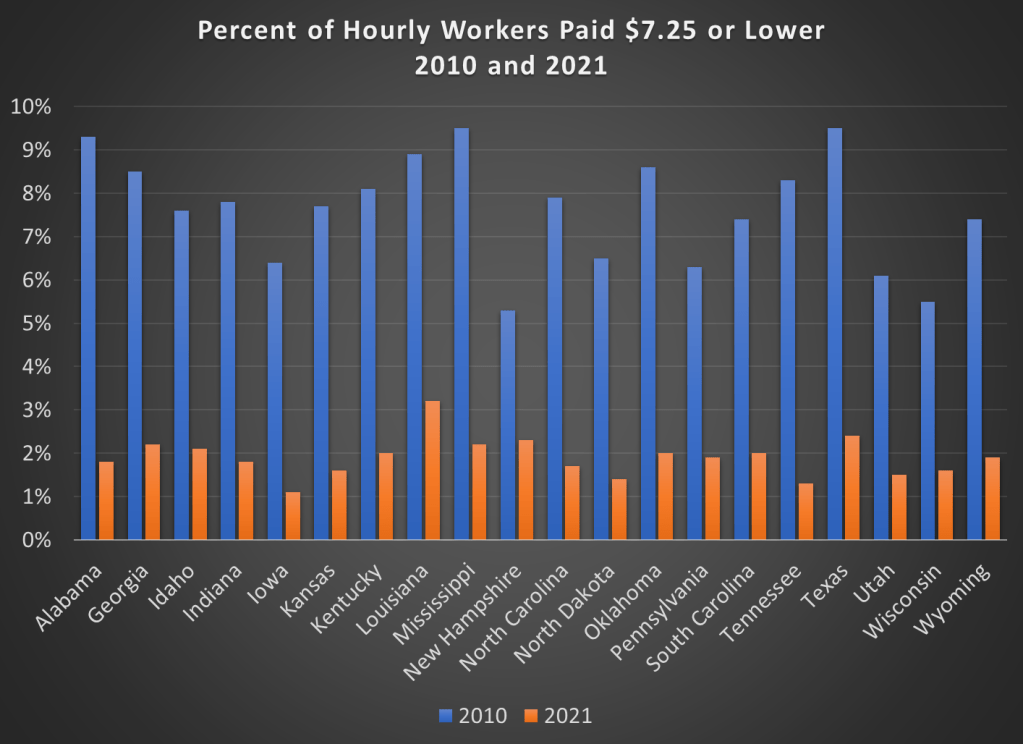
70,000: that’s the number of adults (age 25 and older) in the US that earned the federal minimum wage of $7.25 per hour in 2021.
Another 538,000 adults reported earning below the minimum wage, but these are likely to be workers that earn tips, which aren’t reported in their hourly wages. Legally, they must make at least $7.25 including their tips, though many of them earn more. The data comes from a 2022 report by BLS using CPS data (hopefully the 2023 report is coming out soon).
If we include all workers 16 and older, there are about 1.1 million people earning the federal minimum wage or less. That’s just 1.4% of hourly wage earners, and only 0.8% of all workers (including salaried workers). Crucially, this number has declined dramatically over time from a high of 15.1% of hourly wage earners (8.9% of all workers) in 1981. It has even declined significantly since 2010, the first full year that the $7.25 federal minimum was in effect, when 6% of hourly wage earners (3.5% of all workers) earned $7.25 or lower.
Perhaps, though, a big part of this decline is because most states (and even some cities and counties) now have minimum wages that are above the federal level, in some cases significantly above. Today, only 20 states use the federal minimum wage. No doubt this is important!
However, even if we focus just on those 20 states that use $7.25 per hour as the minimum, there were also large declines in the percent of hourly wage earners that earned $7.25 or less. Some states declined by 7 percentage points or more from 2010 to 2021, though all declined by at least 3 percentage points.
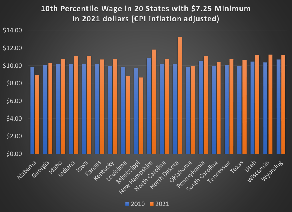
But maybe what’s going on is that employers are just providing wage increases that keep up with price inflation. So while fewer workers are earning the federal minimum wage, maybe they are no better off. We can address that possibility using BLS’s occupational wage data, which allows us to look at wages at the 10th percentile (these aren’t exactly minimum wage earners, but they are close). Real wage declines did happen in a few states (Alabama, Louisiana, and Mississippi), but most of these states experienced clear real wage growth from 2010 to 2021 at the 10th percentile of earners.
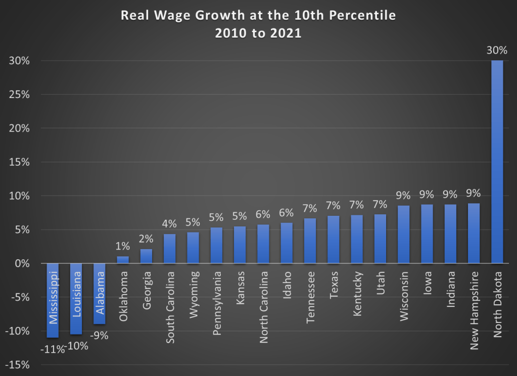
Here are the changes in percentage terms (once again, adjusted for CPI inflation).
Some might look at this growing irrelevance of the minimum wage as a reason to increase the federal minimum wage. But as the data from most states suggests, there are clear increases in wages happening already, suggesting that these are competitive labor markets. The case for raising the legal minimum wage in a competitive labor market is weak (it is stronger in a monopsony labor market).
Here I will draw on a recent article Leads And Lags: Timing A Recession by Seeking Alpha author Eric Basmajian. His overall points are (1) that some indicators are associated with leading segments of the economy (which have historically turned down well before the rest), while others are more lagging, and (2) the leading indicators are strongly flashing recession. Direct quotes from his article are in italics.
Leading Economy, Cyclical Economy & Total Economy
When economic data is released, the information should be contextualized based on where the data point falls in the economic cycle sequence.
We can separate the economy into three buckets: the Leading Economy, the Cyclical Economy, and the Total Economy.
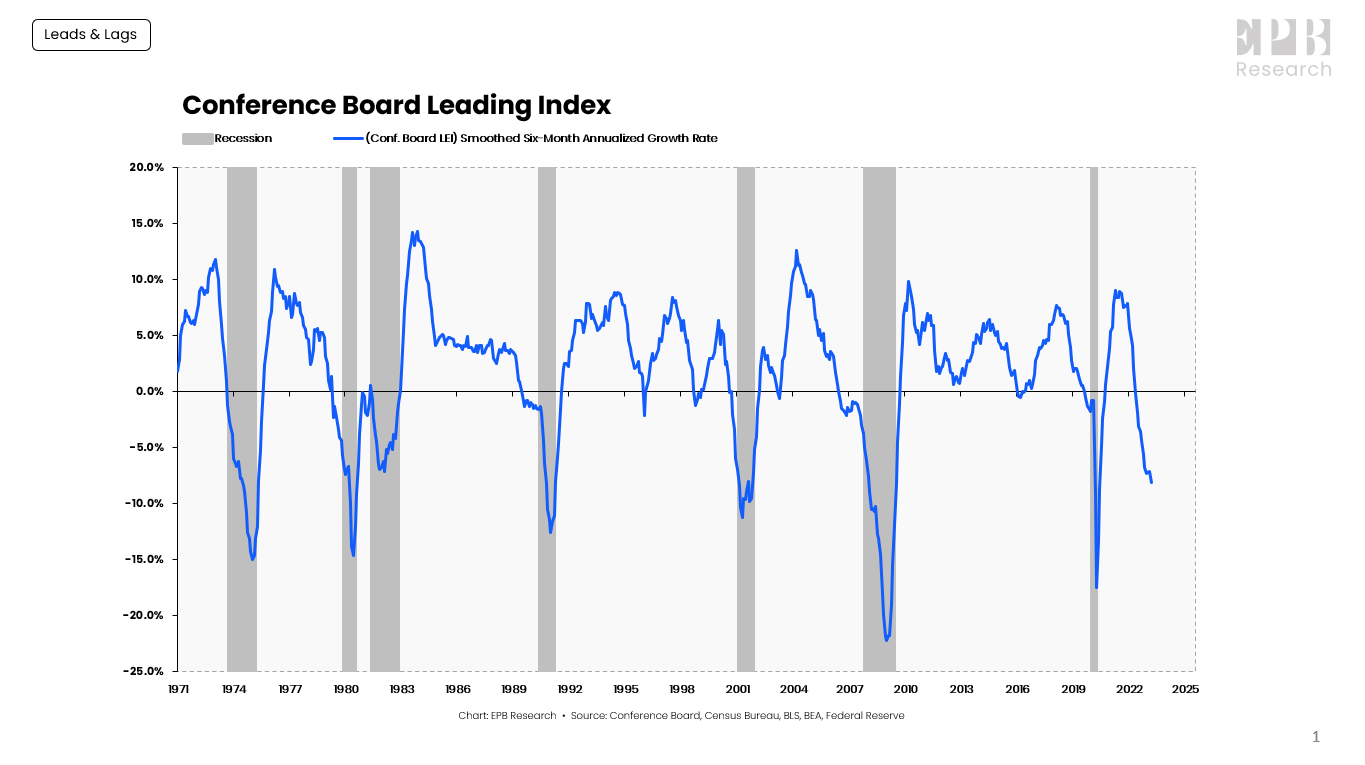
The Leading Economy is defined by the Conference Board Leading Index, which is a basket of ten leading economic variables such as building permits, new orders, and stock prices.
The Leading Index has turned negative before every recession, without exception.
Conference Board, Census Bureau, BLS, BEA, Federal Reserve
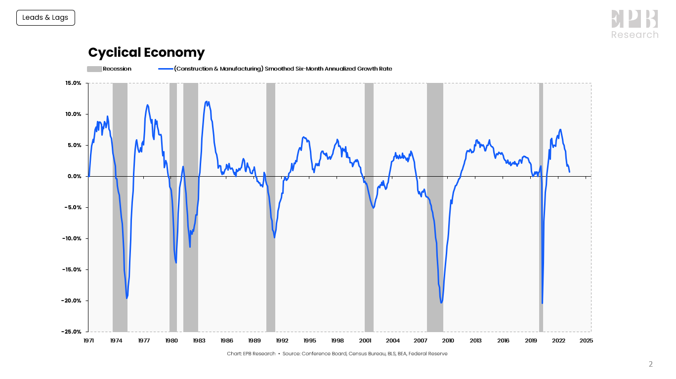
The Cyclical Economy represents the construction and manufacturing sectors. The Cyclical Economy is the driving force behind recessions, always turning negative before the Total Economy, and never giving a false signal; when the Cyclical Economy turns negative, the Total Economy turns negative several months later.
Conference Board, Census Bureau, BLS, BEA, Federal Reserve
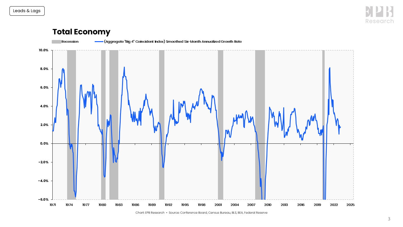
The Total Economy is defined by the “Big-4” Coincident Indicators of economic activity. Nonfarm payrolls, real personal income less transfer payments, real personal consumption, and industrial production are four major economic indicators that the NBER uses as the core of their recession dating procedure.
Conference Board, Census Bureau, BLS, BEA, Federal Reserve
A sustained contraction in the “Big-4” Coincident Indicators is the definition of a recession.
The Total Economy starts showing contracting growth rates about four months into the recession.
Could This Time Be Different?
If we do finally get a recession, it will be probably the most long-expected recession ever. Pundits have been warning for over a year that the Fed’s well-telegraphed program of rate hikes will crater the economy, as the only way to tame inflation.
According to Basmajian, When the Leading Economy and Cyclical Economy are both lower than -1%, a recession, as dated by the NBER, occurred an average of 5 months later, with a range of a 4-month lag to a 14-month lead.
His Leading indicator went negative about 11 months ago (June, 2022). However, it looks like the economy is still humming along and employment remains robust. His Cyclic Economy is on track to go negative right about now, but that has an unusually long lag between Leading and Cyclical:
The Cyclical Economy will likely turn negative with April data and potentially below -1% by May data should the current downward slope remain.
That would push the lag between the Leading Economy and the Cyclical Economy to 11 months, the longest on record.
And the lag before we finally get a bona fide recession in the Total Economy may keep dragging out longer yet. There is even a possible Soft Landing scenario where the rate hikes manage to cool the economy down without causing a severe recession at all.
It seems to me that we collectively are still spending down our excess pandemic benefits, and no recession will come till we finish running through those monies.
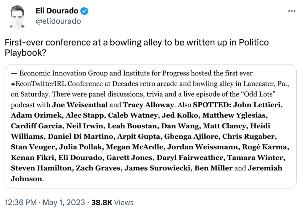
Last weekend fellow Temple University economics PhD Adam Ozimek hosted the inaugural #EconTwitterIRL conference. He managed to get 100+ people, including many big names, to come to his bowling alley / arcade in Lancaster, PA.
The overall demographic of Econ Twitter people appears to be youngish professionals, mostly male, surprisingly social and normal-looking (surprising to me because I retain the ’90s-era stereotype that people who write a lot online are nerds who don’t want to talk to anyone IRL).
Adam opened with a history of EconTwitter, which to him is not just about Twitter, but is anywhere where communities of people write about economics online. This starts with the comment sections of the earliest blogs, like Brad DeLong’s, in the early 2000’s. Then in the late 2000’s many commenters start their own blogs, like Karl Smith at Modeled Behavior. In the 2010’s Econ Twitter comes into its own. It may persist or a new forum might take over, but either way the discussion and community will live on.
While it was cool to see a live recording of Odd Lots, and a panel on innovation with MacArthur Genius Heidi Williams, my favorite panel was the one on immigration, because it saw the most serious disagreement. Garett Jones and Daniel Di Martino argued for reforms to the immigration system that would move it away from a focus on family reunification and toward a focus on skills and other indications (like country of origin) that immigrants would benefit the US economy. In contrast, Leah Boustan argued that the current system has worked well, including for assimilation and economic growth, and we should be wary of making big changes to it. Moderator Cardiff Garcia pointed out the oddity of the economists from George Mason and the Manhattan Institute arguing for a “socialist” system where the government determines what the economy needs when it comes to immigration, while the Princeton economist argues against. Garett Jones noted that the rest of his department at Mason disagree with him, but he’s glad to have the freedom to disagree.
While the panel saw intense disagreement about what the ideal system looks like, all panelists shared a frustration with parts of the current system that seem to pointlessly slow or prevent high-skill immigration. Some of this is bureaucracy slowing the process for immigrants who are legally allowed already. Some is politicians refusing to make the smallest, simplest, most common-sense fixes unless they are part of a comprehensive immigration reform that hits their big priority. The big priorities differ by party, but the commitment to holding simple fixes hostage is bipartisan.
Hopefully discussions like this can start to change things. That might sound naive or idealistic, but on an earlier panel Matt Yglesias noted that we should be both impressed and slightly scared of how aware Capitol Hill staffers are about the opinions of Econ Twitter.
Source. Got 2nd at trivia as part of team Acemoglu et al (actual Acemoglu not included).
The magic of all this is that you never know what can come from a post. You might make a friend, make an enemy, get a job, lose a job, influence public policy, get a job in the White House… even make (or lose) a million dollars. So we keep poasting, and once in a while see the results IRL.
Kevin Erdmann has written a detailed and thoughtful response to my post from last week on housing spending as a percent of income. My goal in that post was to look at consumer spending as a percent of income for a variety of different sub-groups (my primary interest was by age group, but I tried to get into more detail for other sub-groups).
As Erdmann emphasizes in his post, I left out one set of sub-groups that the CEX data allows us to use: renters vs. homeowners. And these are very important groups to look at, since for homeowners (as he points out) many of the costs are implicit (such as the opportunity cost of those that don’t have a mortgage). Lumping all of these households together may obscure some of the different trends.
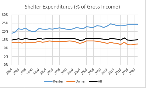
Be sure to read Erdmann’s post in full (he says many smart and correct things), but the key result is in his Figure 2 (reproduced here). Renters have seen the share of their income spent on shelter rise from 19% in 1984 to 24% in 2021. This is not a trivial increase. Owners, by contrast, have seen their share of spending fall, which is how it all gets washed out in the average.
I will concede that Erdmann is probably right on many of his many points. Still, I wanted to see this at a much finer level of detail, since national aggregates might be giving us confusing results. The micro-data in the CEX is probably not detailed enough to give us good breakdowns by MSA.
Apart from some possible geopolitical upset (and theater with the debt ceiling), the Big Issue for the larger economy, and for investing decisions, remains how fast inflation will decline – since that governs how soon the Fed can relent on keeping interest rates high. Those high interest rates are having all kinds of knock-on effects, including bank failures and suppressed home sales.
The investing market seems to be pricing in expectations of significant Fed rate cuts before the end of 2023, which in turn presupposes that inflation will have ratcheted downwards far enough by then to allow the Fed to declare victory. Goods inflation (= mainly stuff made in China) has declined nicely, but services (which comprise the majority of household spending) remains high. It is coming down, but too slowly to realistically hit the Fed’s 2% target this year.
In an article in the Seeking Alpha site title Services Inflation Is Stuck, the investment firm Blackrock notes some technical factors that will likely keep services inflation high for at least the remainder of this year. I will paste in their text in italics:
Core Services ex-Shelter inflation is a bit of a hodgepodge that includes things like medical care services, video and audio services, tuition, and insurance. It comprises roughly a quarter of the CPI basket and, importantly for the Fed, is very domestically oriented.
A key insight from this article is that nearly two-thirds of this key “Core Services ex-Shelter” component consists of:
(1) Service prices that are regulated (especially insurance), and
(2) Services with infrequent price resets (such as tuition and especially medical services):
There are technical factors that make it likely that these particular items will see ongoing, sticky inflation:
Impact of Regulated Prices
Regulated prices tend to be more discrete and more lagged in their changes due to bureaucratic delays and their negotiated nature. Some types of regulated prices, like postage or water and sewage fees, are easily recognizable as subject to government regulation. Somewhat less intuitive is the degree to which insurance in the United States is a regulated price. Insurance comprises the largest share of Core Services ex-Shelter basket and state-level insurance commissioners play important roles in negotiating auto, property, and casualty insurance price changes.
The underwriting costs of insurance have been surging globally – a combination of higher reinsurance premiums, inflated asset values, and more natural disasters. These rising costs have only just begun to flow through into consumer prices; auto insurance costs were an upside surprise within March’s CPI report.
Jumps in Medical and Education Prices Will Appear Later
Though the market has been fixated on the painstaking details of the month-over-month inflation prints, many of the sub-components of the CPI do not update monthly. Two of the more important items within the core services basket – medical care services and tuition – only update their prices annually. Coincidentally, updates for both of these categories take place in the autumn, and both are set to rise strongly.
Medical care services are the largest component (28%) of Core Services ex-Shelter, but have a complex and lagged computation and update only once a year in October. Medical services inflation has been negative since last October as a consequence of excess consumer demand for post-pandemic doctors’ visits, however, we expect this mechanical effect will abate later this year and thereafter lift core services inflation.
Tuition is another example of a service with intermittent price resets, given prices are set on the basis of the academic year. We expect the broad-based upward wage pressure in education to be passed through to higher education consumer prices later this year when students return to school.
And so…I expect “higher for longer” inflation and interest rates.
I’m currently purchasing a new house and I want to share some insights. Baseline knowledge: Houses are unique goods on multiple margins that are imperfect substitutes. Let’s assume that both a buyer and a seller have real estate agents in the USA. The opportunity cost to the buyer is selecting another house that is not quite as desirable or finding a comparably desirable house after a wait (due to time searching and the appearance of new listings). Legally, the seller is not allowed to lie about the property details (though they can claim ignorance). The lending process makes it difficult for the buyer to lie.
Step 1: List and Bid
The seller chooses a price low enough that will permit a sale within their preferred timeframe, and high enough so that they earn a commensurate return. There is a tradeoff.
The buyer makes an offer. Before buying, I thought that the offer was, more or less, just bidding a price. That would make the problem nice and 1-dimensional. It would fit nicely into the auction theory that I learned in grad school. But that’s not the whole story. As it turns out, an offer specifies other details too. It specifies:
The price.
Earnest money. This is the amount that the buyers pays immediately in order to signal legitimate interest in the property. It’s often held in escrow by a 3rd party in order to improve credibility.
The number of days until closing (signing the final contract).
The number of days for ‘due diligence’. This is the period during which inspections must/can be done. The seller or their agent must make the house reasonably available for inspection during this period.
The appraisal period. This is the length of time during which an appraisal of the property determines the value of the home insofar as a lending institution is concerned. Without a loan, this number can be zero is irrelevant.
A lender’s pre-approval letter specifying the permitted size of the loan and the down payment. This is a signal of credibility that the buyer is able to pay. The buyer can request to be approved for a smaller loan in order to signal unwillingness to pay more.
Any contingencies, such as whether another property must sell first, or a delay is requested. Really, this can be almost anything that the buyer wants. Some people get creative in their offers, like paying a higher price in exchange for a later closing date or rent-to-own contracts.
Given the above details, a potential buyer would like to craft the offer to meet the seller’s preferences while also acknowledging the scarcity of the buyer’s resources. As it turns out, not all resources are instantly convertible. One may be willing to move quickly but have a lower budget. Or, be willing to pay a higher price, contingent on the sale of another property.


