Today I’ll go into more detail on several measures of the labor force, but I won’t only compare it to 2019. I’ll compare it to all available data. And the sum total of the data suggests the 2023 was one of the best years for the US labor market on record. Note: December 2023 data isn’t available until January 5th, so I’m jumping the gun a little bit. I’m going to assume December looks much like November. We can revisit in 2 weeks if that was wrong.
The Unemployment Rate has been under 4% for the entire year. The last time this happened (date goes back to 1948) was 1969, though 2022 and 2019 were both very close (just one month at 4%). In fact, the entire period from 1965-1969 was 4% or less, though following January 1970 there wasn’t single month under 4% under the year 2000!
Like GDP, the Unemployment Rate is one of the broadest and most widely used macro measures we have, but they are also often criticized for their shortcomings, as I wrote in an April 2023 post.
With that in mind, let’s look to some other measures of the labor market.
Boaz Weinstein is a really smart guy. At age 16 the US Chess Federation conferred on him the second highest (“Life Master”) of the eight master ratings. As a junior in high school, he won a stock-picking contest sponsored by Newsday, beating out a field of about 5000 students. He started interning with Merrill Lynch at age 15, during summer breaks. He has the honor of being blacklisted at casinos for his ability to count cards.
He entered into heavy duty financial trading right out of college, and quickly became a rock star. He joined international investment bank Deutsche Bank in 1998, and led their trading of then-esoteric credit default swaps (securities that payout when borrowers default). Within a few years his group was managing some $30 billion in positions, and typically netting hundreds of millions in profits per year. In 2001, Weinstein was named a managing director of the company, at the tender age of 27.
Weinstein left Deutsche Bank in 2009 and started his own credit-focused hedge fund, Saba Capital Management. One of its many coups was to identify some massive, seemingly irrational trades in 2012 that were skewing the credit default markets. Weinstein pounced early, and made bank by taking the opposite sides of these trades. He let other traders in on the secret, and they also took opposing positions.
(It turned out these huge trades were made by a trader in J. P. Morgan’s London trading office, Bruno Iksil, who was nick-named the London Whale. Morgan’s losses from Iksil’s trades mounted to some $6.2 billion.)
For what it’s worth, Weinstein is by all accounts a really nice guy. This is not necessarily typical for many high-powered Wall Street traders who have been as successful as he.
Weinstein and the Sprawling World of Closed End Funds
If you have a brokerage account, you can buy individual securities, like Microsoft common stock shares, or bonds issued by General Motors. Many investors would prefer not to have to do the work of screening and buying and holding hundreds of stocks or bonds. No problem, there exist many funds, which do all the work for you. For instance, the SPY fund holds shares of all 500 large-cap American companies that are in the S&P 500 index, so you can simply buy shares of the one fund, SPY.
Without going too deeply into all this, there are three main types of funds held by retail investors. These are traditional open-end mutual funds, the more common exchange-traded funds (ETFs), and closed end funds (CEFs). CEFs come in many flavors, with some holding plain stocks, and others holding high-yield bonds or loans, or less-common assets like spicy CLO securities. A distinctive feature of CEFs is that the market price per share often differs from the net asset value (NAV) per share. A CEF may trade at a premium or a discount to NAV, and that premium or discount can vary widely with time and among otherwise-similar funds. This makes optimal investing in CEFs very complex, but potentially-rewarding: if you can keep rotating among CEF’s, buying ones that are heavily discounted, then selling them when the discount closes, you can in theory do much better than a simple buy and hold investor.
I played around in this area, but did not want to devote the time and attention to doing it well, considering I only wanted to devote 3-4% of my personal portfolio to CEFs. There are over 400 closed end funds out there. So, I looked into funds whose managers would (for a small fee) do that optimized buying and selling of CEFs for me.
It turns out that there are several such funds-of-CEF-funds. These include ETFs with the symbols YYY and PCEF, CEFS, and also the closed end funds FOF and RIV. YYY and PCEF tend to operate passively, using fairly mechanical rules. PCEF aims to simply replicate a broad-based index of the CEF universe, while YYY rebalances periodically to replicate an “intelligent” index which ranks CEFs by yield, discount to net asset value and liquidity. FOF holds and adjusts a basket of undervalued CEFs chosen by active managers, while RIV holds a diverse pot of high-yield securities, including CEFs. The consensus among most advisers I follow is that FOF is a decent buy when it is trading at a significant discount, but it makes no sense to buy it now, when it is at a relatively high premium; you would be better off just buying a basket of CEFs yourself.
I settled on using CEFS (Saba Closed-End Funds ETF) for my closed end fund exposure. It is very actively co-managed by Saba Capital Management, which is headed by none other than Boaz Weinstein. I trust whatever team he puts together. Among other things, Saba will buy shares in a CEF that trades at a discount, then pressure that fund’s management to take actions to close the discount.
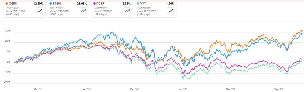
The results speak for themselves. Here is a plot of CEFS (orange line) versus SP500 index (blue), and two passively-managed ETFs that hold CEFs, PCEF (purple) and YYY (green) over the past three years:
The Y axis is total return (price action plus reinvestment of dividends). CEFS smoked the other two funds-of-funds, and even edged out the S&P in this time period. It currently pays out a juicy 9% annualized distribution. Thank you, Mr. Weinstein, and Merry Christmas to all my fellow investors.
Boilerplate disclaimer: Nothing in this article should be regarded as advice to buy or sell any security.
Whether it’s a high holiday or just a nice day to get Chinese food with your family and watch old movies, I hope you all have the very best Christmas possible, no matter what that means for you. But do take the day off if at all possible and, if the opportunity arises, make it a little easier for those who can’t.
I have a paper that emphasizes ChatGPT errors. It is important to recognize that LLMs can make mistakes. However, someone could look at our data and emphasize the opposite potential interpretation. On many points, and even when coming up with citations, the LLM generated correct sentences. More than half of the content was good.
Apparently, LLMs just solved an unsolvable math problem. Is there anything they can’t do? Considering how much of human expression and culture revolves around religion, we can expect AI’s to get involved in that aspect of life.
Alex thinks it will be a short hop from Personal Jesus Chatbot to a whole new AI religion. We’ll see. People have had “LLMs” in the form of human pastors, shaman, or rabbis for a long time, and yet sticking to one sacred text for reference has been stable. I think people might feel the same way in the AI era – stick to the canon for a common point of reference. Text written before the AI era will be considered special for a long time, I predict. Even AI’s ought to be suspicious of AI-generated content, just in the way that humans are now (or are they?).
Many religious traditions have lots of training literature. (In our ChatGPT errors paper, we expect LLMs to produce reliable content on topics for which there is plentiful training literature.)
I gave ChatGPT this prompt:
Can you write a Bible study? I’d like this to be appropriate for the season of Advent, but I’d like most of the Bible readings to be from the book of Job. I’d like to consider what Job was going through, because he was trying to understand the human condition and our relationship to God before the idea of Jesus. Job had a conception of the goodness of God, but he didn’t have the hope of the Gospel. Can you work with that?
The Differences-in-Differences literature has blown up in the past several years. “Differences-in-Differences” refers to a statistical method that can be used to identify causal relationships (DID hereafter). If you’re interested in using the new methods in Stata, or just interested in what the big deal is, then this post is for you.
First, there’s the basic regression model where we have variables for time, treatment, and a variable that is the product of both. It looks like this:
The idea is that that there is that we can estimate the effect of time passing separately from the effect of the treatment. That allows us to ‘take out’ the effect of time’s passage and focus only on the effect of some treatment. Below is a common way of representing what’s going on in matrix form where the estimated y, yhat, is in each cell.
Each quadrant includes the estimated value for people who exist in each category. For the moment, let’s assume a one-time wave of treatment intervention that is applied to a subsample. That means that there is no one who is treated in the initial period. If the treatment was assigned randomly, then β=0 and we can simply use the differences between the two groups at time=1. But even if β≠0, then that difference between the treated and untreated groups at time=1 includes both the estimated effect of the treatment intervention and the effect of having already been treated prior to the intervention. In order to find the effect of the intervention, we need to take the 2nd difference. δ is the effect of the intervention. That’s what we want to know. We have δ and can start enacting policy and prescribing behavioral changes.
Easy Peasy Lemon Squeezy. Except… What if the treatment timing is different and those different treatment cohorts have different treatment effects (heterogeneous effects)?* What if the treatment effects change over time the longer an individual is treated (dynamic effects)**? Further, what if the there are non-parallel pre-existing time trends between the treated and untreated groups (non-parallel trends)?*** Are there design changes that allow us to estimate effects even if there are different time trends?**** There’re more problems, but these are enough for more than one blog post.
For the moment, I’ll focus on just the problem of non-parallel time trends.
What if untreated and the to-be-treated had different pre-treatment trends? Then, using the above design, the estimated δ doesn’t just measure the effect of the treatment intervention, it also detects the effect of the different time trend. In other words, if the treated group outcomes were already on a non-parallel trajectory with the untreated group, then it’s possible that the estimated δ is not at all the causal effect of the treatment, and that it’s partially or entirely detecting the different pre-existing trajectory.
Below are 3 figures. The first two show the causal interpretation of δ in which β=0 and β≠0. The 3rd illustrates how our estimated value of δ fails to be causal if there are non-parallel time trends between the treated and untreated groups. For ease, I’ve made β=0 in the 3rd graph (though it need not be – the graph is just messier). Note that the trends are not parallel and that the true δ differs from the estimated delta. Also important is that the direction of the bias is unknown without knowing the time trend for the treated group. It’s possible for the estimated δ to be positive or negative or zero, regardless of the true delta. This makes knowing the time trends really important.
STATA Implementation
If you’re worried about the problems that I mention above the short answer is that you want to install csdid2. This is the updated version of csdid & drdid. These allow us to address the first 3 asterisked threats to research design that I noted above (and more!). You can install these by running the below code:
program fra
    syntax anything, [all replace force]
    local from "https://friosavila.github.io/stpackages"
    tokenize `anything'
    if "`1'`2'"==""  net from `from'
    else if !inlist("`1'","describe", "install", "get") {
        display as error "`1' invalid subcommand"
    }
    else {
        net `1' `2', `all' `replace' from(`from')
    }
    qui:net from http://www.stata.com/
end
fra install fra, replace
fra install csdid2
ssc install coefplot
Once you have the methods installed, let’s examine an example by using the below code for a data set. The particulars of what we’re measuring aren’t important. I just want to get you started with the an application of the method.
local mixtape https://raw.githubusercontent.com/Mixtape-Sessions
use `mixtape'/Advanced-DID/main/Exercises/Data/ehec_data.dta, clear
qui sum year, meanonly
replace yexp2 = cond(mi(yexp2), r(max) + 1, yexp2)
The csdid2 command is nice. You can use it to create an event study where stfips is the individual identifier, year is the time variable, and yexp2 denotes the times of treatment (the treatment cohorts).
The above output shows us many things, but I’ll address only a few of them. It shows us how treated individuals differ from not-yet treated individuals relative to the time just before the initial treatment. In the above table, we can see that the pre-treatment average effect is not statistically different from zero. We fail to reject the hypothesis that the treatment group pre-treatment average was identical to the not-yet treated average at the same time period. Hurrah! That’s good evidence for a significant effect of our treatment intervention. But… Those 8 preceding periods are all negative. That’s a little concerning. We can test the joint significance of those periods:
estat event, revent(-8/-1)
Uh oh. That small p-value means that the level of the 8 pretreatment periods significantly deviate from zero. Further, if you squint just a little, the coefficients appear to have a positive slope such that the post-treatment values would have been positive even without the treatment if the trend had continued. So, what now?
Wouldn’t it be cool if we knew the alternative scenario in which the treated individuals had not been treated? That’s the standard against which we’d test the observed post-treatment effects. Alas, we can’t see what didn’t happen. BUT, asserting some premises makes the job easier. Let’s say that the pre-treatment trend, whatever it is, would have continued had the treatment not been applied. That’s where the honestdid stata package comes in. Here’s the installation code:
local github https://raw.githubusercontent.com
net install honestdid, from(`github'/mcaceresb/stata-honestdid/main) replace
honestdid _plugin_check
What does this package do? It does exactly what we need. It assumes that the pre-treatment trend of the prior 8 periods continues, and then tests whether one or more post-treatment coefficients deviate from that trend. Further, as a matter of robustness, the trend that acts as the standard for comparison is allowed to deviate from the pre-treatment trend by a multiple, M, of the maximum pretreatment deviations from trend. If that’s kind of wonky – just imagine a cone that continues from the pre-treatment trend that plots the null hypotheses. Larger M’s imply larger cones. Let’s test to see whether the time-zero effect significantly differs from zero.
What does the above table tell us? It gives us several values of M and the confidence interval for the difference between the coefficient and the trend at the 95% level of confidence. The first CI is the original time-0 coefficient. When M is zero, then the null assumes the same linear trend as during the pretreatment. Again, M is the ratio by which maximum deviations from the trend during the pretreatment are used as the null hypothesis during the post-treatment period. So, above, we can see that the initial treatment effect deviates from the linear pretreatment trend. However, if our standard is the maximum deviation from trend that existed prior to the treatment, then we find that the alpha is just barely greater than 0.05 (because the CI just barely includes zero).
That’s the process. Of course, robustness checks are necessary and there are plenty of margins for kicking the tires. One can vary the pre-treatment periods which determine the pre-trend, which post-treatment coefficient(s) to test, and the value of M that should be the standard for inference. The creators of the honestdid seem to like the standard of identifying the minimum M at which the coefficient fails to be significant. I suspect that further updates to the program will come along that spits that specific number out by default.
I’ve left a lot out of the DID discussion and why it’s such a big deal. But I wanted to share some of what I’ve learned recently with an easy-to-implement example. Do you have questions, comments, or suggestions? Please let me know in the comments below.
The above code and description is heavily based on the original author’s support documentation and my own Statalist post. You can read more at the above links and the below references.
*Sun, Liyang, and Sarah Abraham. 2021. “Estimating Dynamic Treatment Effects in Event Studies with Heterogeneous Treatment Effects.” Journal of Econometrics, Themed Issue: Treatment Effect 1, 225 (2): 175–99. https://doi.org/10.1016/j.jeconom.2020.09.006.
**Sant’Anna, Pedro H. C., and Jun Zhao. 2020. “Doubly Robust Difference-in-Differences Estimators.” Journal of Econometrics 219 (1): 101–22. https://doi.org/10.1016/j.jeconom.2020.06.003.
***Callaway, Brantly, and Pedro H. C. Santa Anna. 2021. “Difference-in-Differences with Multiple Time Periods.” Journal of Econometrics, Themed Issue: Treatment Effect 1, 225 (2): 200–230. https://doi.org/10.1016/j.jeconom.2020.12.001.
****Rambachan, Ashesh, and Jonathan Roth. 2023. “A More Credible Approach to Parallel Trends.” The Review of Economic Studies 90 (5): 2555–91. https://doi.org/10.1093/restud/rdad018.
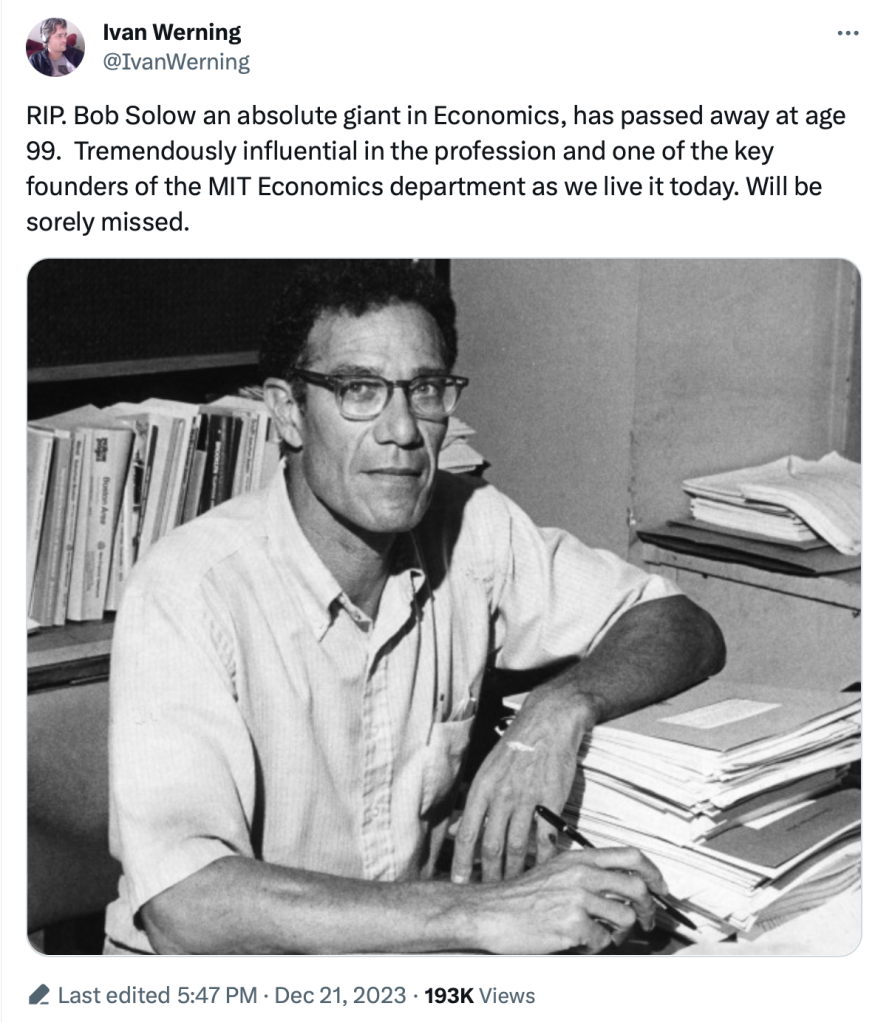
2023 continues to be a dangerous year for eminent economists. We have once again lost a Nobel laureate who was influential even by the standard of Nobelists, Robert Solow:
I’m sure you will soon see many tributes that discuss his namesake Solow Model (MR already has one), or discuss him as a person. I never got to meet him (just saw him give a talk) and the Solow Model is well known, so I thought I’d take this occasion to discuss one of his lesser-known papers- “Sustainability: An Economists Perspective“. What follows comes from my 2009 reaction to his paper:
Lately many journalists and folks on X/Twitter have pointed out a seeming disconnect: by almost any normal indicator, the US economy is doing just fine (possibly good or great). But Americans still seem dissatisfied with the economy. I wanted to put all the data showing this disconnect into one post.
In particular, let’s make a comparison between November 2019 and November 2023 economic data (in some cases 2019q3 and 2023q3) to see how much things have changed. Or haven’t changed. For many indicators, it’s remarkable how similar things are to probably the last month before anyone most normal people ever heard the word “coronavirus.”
First, let’s start with “how people think the economy is doing.” Here’s two surveys that go back far enough:
The University of Michigan survey of Consumer Sentiment is a very long running survey, going back to the 1950s. In November 2019 it was at roughly the highest it had ever been, with the exception of the late 1990s. The reading for 2023 is much, much lower. A reading close to 60 is something you almost never see outside of recessions.
The Civiqs survey doesn’t go back as far as the Michigan survey, but it does provide very detailed, real-time assessments of what Americans are thinking about the economy. And they think it’s much worse than November 2019. More Americans rate the economy as “very bad” (about 40%) than the sum of “fairly good” and “very good” (33%). The two surveys are very much in alignment, and others show the same thing.
I’m on Bluesky. I’m on twitter/X. I’m not happy with either right now. I wasn’t particularly happy on twitter before, but that was before it became much worse, so now I wish it could back to the way it was, when I was also complaining, because it turns out the counterfactual universe where it was different is actually worse. So here we are.
The decline in my personal portfolio of social media largely comes down to critical mass. The decline in Twitter usage has reduced its value to me (and most of its users). Only a tiny fraction of this loss in Twitter value is offset by the value I receive from Bluesky for the simple reason it doesn’t have enough users. Even if 100% of Twitter exits had led to Bluesky entrants, it would still be a value loss because the marginal user currently offers more value at Twitter. Standard network goods, returns to scale, power law mechanics, yada yada yada.
Now, to be clear, Twitter is still well above the minimum critical mass threshold for significant value-add, but the good itself has also been damaged by Elon’s managerial buffoonery. Bluesky, depending on your point of view and consumer niche, hasn’t achieved a self-sustaining critical mass (e.g. econsky hasn’t quite cracked it, unfortunately). The result is a decent number of people half-committing to both, which only serves to undermine consumer value being generated in the entire “microblogging” social media space.
The problem, simply put, is that Twitter still has too much option value to leave entirely. If (when) Elon get’s the mother-of-all-margin-calls, he’ll likely have to sell Twitter or large amount of his Tesla holdings. If he’s smart and doesn’t cave in to the sunk cost fallacy (a non-trivial “if”), he’ll sell Twitter. If new ownership successfully returns Twitter to suitable fascimile of it’s previous form, people will come flooding back, Bluesky will turn-off or wholly adapt into a new consumer paradigm, and everyone will be thrilled to have squatted on their previous accounts.
If Twitter retains its current form, then it will probably die, though not at the direct hands of Bluesky. More likely it will be displaced by some new product most of us don’t yet see coming, as the next generation departs twitter the way millenials departed Facebook for Snapchat and, eventually, TikTok. Perhaps counterintuitively, this outcome is actually excellent for Bluesky, because the absence of twitter will send the 3% of “professional” twitter users (economists, journalists, thinktank wonks, policy makers, etc) to Bluesky, where they will achieve niche critical mass and live happily ever after (at least as happy as one can be whilst immersed in a sea of status-obsessed try-hards).
But for the moment, we’re all a little stuck trying to make do with finding fulfillment in the complex personal lives, loving families, transcendant art, and multidimensional experiences that remain confined to meatspace. We can only do our best and remain strong during such trying times.
Back in June, I watched the livestream of the Chapman Economic Forecast with Dr. Jim Doti (who was president when I was a student at Chapman). Typically, this is a valuable informative event, and the team has an excellent record of performance. They have often outdone other forecasters in predicting the future.
That is why I feel a little bad for making this post in the summer and tweeting out Doti’s prediction that we would have a recession by now.
To be fair to Doti, there has been a lot of uproar over this issue. Lots of people thought the economy would be bad. And lots of people feel like the economy is bad (the “vibecession”) even though it is objectively not. Many tweets have gone by about it.
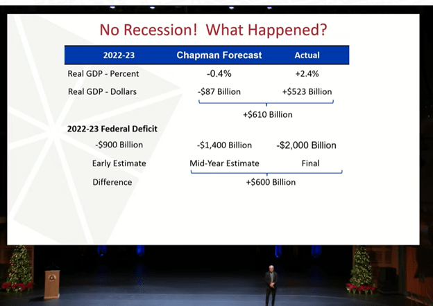
Doti opened by saying his prediction had turned out to be wrong. He had an explanation for it (pictured below). You can watch it free here (recorded on Dec 14).
Doti said that he had expected a large fiscal stimulus in the form of deficit spending, however he had not expected the deficit to be so large. Debt-financed spending propped up an economy that was otherwise poised to contract. At least, that is a plausible story.
Looking forward, Doti does not predict a recession next year, but he does predict weak growth and possibly one quarter of GPD decline (not two).
The next part of talk was about the long-term consequences of deficit spending. Nothing is free. TANSTAAFL
In addition to vibecession, anyone following economics in 2023 needs to know what a “soft landing” is.
Fed Chair Powell: "There's little basis for thinking the economy is in a recession now."
The latest Fed projections show a soft landing in 2024.
Growth slowing, but positive +1.4% Inflation cooling to ~2.4% Unemployment rising to 4.1% (so just below recession trigger) pic.twitter.com/6cvgC6l5Nd
I’ve taught GT a total of 5 time. Below are my average student course evaluations for “I would recommend this class to others” and “I would consider this instructor excellent”. Although the general trend has been improvement, improving ratings and the course along the way, some more context would be helpful. In 2019, my expectations for math were too high. Shame on me. It was also my first time teaching GT, so I had a shaky start. In 2020, I smoothed out a lot of the wrinkles, but I hadn’t yet made it a great class.
In 2021, I had a stellar crop of students. There was not a single student who failed to learn. The class dynamic was perfect and I administered the course even more smoothly. They were comfortable with one another, and we applied the ideas openly. In 2022, things went south. There were too many students enrolled in the section, too many students who weren’t prepared for the course, and too many students who skated by without learning the content. Finally, in 2023, the year of my changes, I had a small class with a nice symmetrical set of student abilities.
Historically, I would often advertise this class, but after the disappointing 2022 performance, and given that I knew that I would be making changes, I didn’t advertise for the 2023 section. That part worked out perfectly. Clearly, there is a lot of random stuff that happens that I can’t control. But, my job is to get students to learn, help the capable students to excel, and to not make students *too* miserable in the process – no matter who is sitting in front of me.