The government continues to be great at collecting data but not so good at sharing it in easy-to-use ways. That’s why I’ve been on a quest to highlight when independent researchers clean up government datasets and make them easier to use, and to clean up such datasets myself when I see no one else doing it; see previous posts on State Life Expectancy Data and the Behavioral Risk Factor Surveillance System.
National Health Expenditure Accounts Historical State Data: The original data from the Centers for Medicare and Medicaid Services on health spending by state and type of provider are actually pretty good as government datasets go: they offer all years (1980-2020) together in a reasonable format (CSV). But it comes in separate files for overall spending, Medicare spending, and Medicaid spending; I merge the variables from all 3 into a single file, transform it from a “wide format” to a “long format” that is easier to analyze in Stata, and in the “enhanced” version I offer inflation-adjusted versions of all spending variables. Excel and Stata versions of these files, together with the code I used to generate them, are here.
A warning to everyone using the data, since it messed me up for a while: in the documentation provided by CMMS, Table 3 provides incorrect codes for most variables. I emailed them about this but who knows when it will get fixed. My version of the data should be correct now, but please let me know if you find otherwise. You can find several other improved datasets, from myself and others, on my data page.
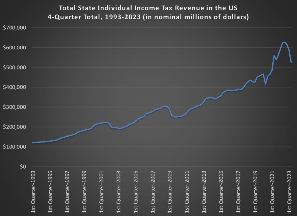
State tax revenue is down a lot since last year. The latest comparable data from Census’s QTAX survey is for the 2nd quarter of 2023, and it shows a massive hit: state tax revenue was down 14% from the same quarter in 2022, which is about $66 billion. Almost all of that decline is from income tax revenue, specifically individual income tax revenue which is down over 30% (almost $60 billion). General sales taxes, the other workhorse of state budgets, is essentially flat over the year.
That’s a huge revenue decline! So, what’s going on? In some states, there has been an attempt to blame recent tax cuts. It’s not a bad place to start, since half of US states have reduced income taxes in the past 3 years, mostly reducing top marginal tax rates. But that can’t be the full explanation, since almost every state saw a reduction in revenue: just 3 states had individual income tax revenue increases (Louisiana, Mississippi, and New Hampshire) from 2022q2 to 2023q2, and they were among the half of states that reduced rates!
To get some perspective let’s look at long-run trends. This chart shows total state individual income tax revenue for all 50 states (sorry, DC) going back to 1993. I use a 4-quarter total, since tax receipts are seasonal (and because states sometimes move tax deadlines due to things like disasters, a specific quarter can sometimes look weird). And importantly, this data is notinflation adjusted. Don’t worry, I will do an adjustment further below in this post, but for starters let’s just look at the nominal dollars, because nominal dollars are how states receive money!
Now, driven by that spending surge, inflation has also surged, and thus the Fed has been obliged to raise interest rates. And so now, in addition to the enormous current deficit spending, that tsunami of short-term debt from 2020-2021 is coming due, to be refinanced at much higher rates. This high interest expense will contribute further to the growing government debt.
Hedge fund manager Stanley Druckenmiller commented in an interview:
When rates were practically zero, every Tom, Dick and Harry in the U.S. refinanced their mortgage… corporations extended [their debt],” he said. “Unfortunately, we had one entity that did not: the U.S. Treasury….
Janet Yellen, I guess because political myopia or whatever, was issuing 2-years at 15 basis points[0.15%] when she could have issued 10-years at 70 basis points [0.70 %] or 30-years at 180 basis points [1.80%],” he said. “I literally think if you go back to Alexander Hamilton, it is the biggest blunder in the history of the Treasury. I have no idea why she has not been called out on this. She has no right to still be in that job.
Unsurprisingly, Yellen pushed back on this charge (unconvincingly). More recently, former Treasury official Amar Reganti has issued a more detailed defense. Here are some excerpts of his points:
( 1 ) …The Treasury’s functions are intimately tied to the dollar’s role as a reserve currency. It is simply not possible to have a reserve currency without a massive supply of short-duration fixed income securities that carry no credit risk.
( 2 ) …For the Treasury to transition the bulk of its issuance primarily to the long end of the yield curve would be self-defeating since it would most likely destabilise fixed income markets. Why? The demand for long end duration simply does not amount to trillions of dollars each year. This is a key reason why the Treasury decided not to issue ultralong bonds at the 50-year or 100-year maturities. Simply put, it did not expect deep continued investor demand at these points on the curve.
( 3 ) …The Treasury has well over $23tn of marketable debt. Typically, in a given year, anywhere from 28% to 40% of that debt comes due…so as not to disturb broader market functioning, it would take the Treasury years to noticeably shift its weighted average maturity even longer.
( 4 ) …The Treasury does not face rollover risk like private sector issuers.
Here is my reaction:
What Reganti says would be generally valid if the trillions of excess T-bond issuance in 2020-2021 were sold into the general public credit market. In that case, yes, it would have been bad to overwhelm the market with more long-term bonds than were desired. But that is simply not what happened. It was the Fed that vacuumed up nearly all those Treasuries, not the markets. The markets were desperate for cash, and hence the Fed was madly buying any and every kind of fixed income security, public and corporate and mortgage (even junk bonds that probably violated the Fed’s bylaws), and exchanging them mainly for cash. Sure, the markets wanted some short-term Treasuries as liquid, safe collateral, but again, most of what the Treasury issued ended up housed in the Fed’s digital vaults.
So, I remain unconvinced that the issuance of mainly long-term (say 10-year and some 30-year; no need to muddy the waters like Reganti did with harping on 50–100-year bonds) debt would have been a problem. So much fixed-income debt was vomited forth from the Treasury that even making a minor portion of it short-term would, I believe, have satisfied market needs. The Fed could have concentrated on buying and holding the longer-term bonds, and rolling them over eventually as needed, without disturbing the markets. That would have bought the country a decade or so of respite before the real interest rate effects of the pandemic debt issuance began to bite.
Did you know you could make a Godzilla movie, maybe the best one at that, for $15 million dollars (or 3 minutes of Chris Pratt in “End Game”, if you’d prefer numeraire)? This film, in which Godzilla is basically the demon baby of Jason Voorhees and the shark from Jaws, deftly explores concepts of guilt, shame, redemption, forgiveness, and family. I cried at the end. I repeat, I cried at the end of a Godzilla movie.
In the last month I’ve watched a Godzilla movie that is specifically constructed to recreate the feeling of a 1950s monster movie, a flawed but admirable attempt to make a modern Charlie Chaplin movie (Fool’s Paradise), and a watchable if uneven and wholly debauched variation on “Singin’ in the Rain” (Babylon). I don’t think this is a coincidence. I think this is a response to VFX and super hero (not comic book) movie fatigue. One way to do that is to go backwards, not in subject matter or setting necessarily, but in story composition and construct. The performances in all three films felt more stage than screen. Texture was emphasized over shock and awe. Emotional crescendos felt more earned than manipulated. I’m not saying these three films are perfect or even necessarily good. What I’m saying is that they felt like a return to older form of film as a medium.
For the last 15 years we’ve had a lot of “remakes” that attempted to modernize old films. Don’t be surprised if we see the inverse going forward: new, original stories filmed in a manner that feels older. “The Thing” but it’s a sea alien on an oil platform, everything wet and on fire. “All the Presidents Men” but it’s a coverup in local Iowa government, with scratchy sunken sofas and life-changing smoke breaks. “Working Girl” but it’s Zendaya and Scarlett Johannsen in a fully modern context, where a misread text subverts an expected plot turn on a broken iPhone screen. Not for a love of classic cinema mind you, or even art, but because making 10 to 1 on winners and losing next to nothing on flops is a business proposition more than a few studios are likely to find enticing.
We study whether people will pay for a fact-check on AI writing. ChatGPT can be very useful, but human readers should not trust every fact that it reports. Yesterday’s post was about ChatGPT writing false things that look real.
The reason participants in our experiment might pay for a fact-check is that they earn bonus payments based on whether they correctly identify errors in a paragraph. If participants believe that the paragraph does not contain any errors, they should not pay for a fact-check. However, if they have doubts, it is rational to pay for a fact-check and earn a smaller bonus, for certain.
Abstract: We explore whether people trust the accuracy of statements produced by large language models (LLMs) versus those written by humans. While LLMs have showcased impressive capabilities in generating text, concerns have been raised regarding the potential for misinformation, bias, or false responses. In this experiment, participants rate the accuracy of statements under different information conditions. Participants who are not explicitly informed of authorship tend to trust statements they believe are human-written more than those attributed to ChatGPT. However, when informed about authorship, participants show equal skepticism towards both human and AI writers. There is an increase in the rate of costly fact-checking by participants who are explicitly informed. These outcomes suggest that trust in AI-generated content is context-dependent.
Our original hypothesis was that people would be more trusting of human writers. That turned out to be only partially true. Participants who are not explicitly informed of authorship tend to trust statements they believe are human-written more than those attributed to ChatGPT.
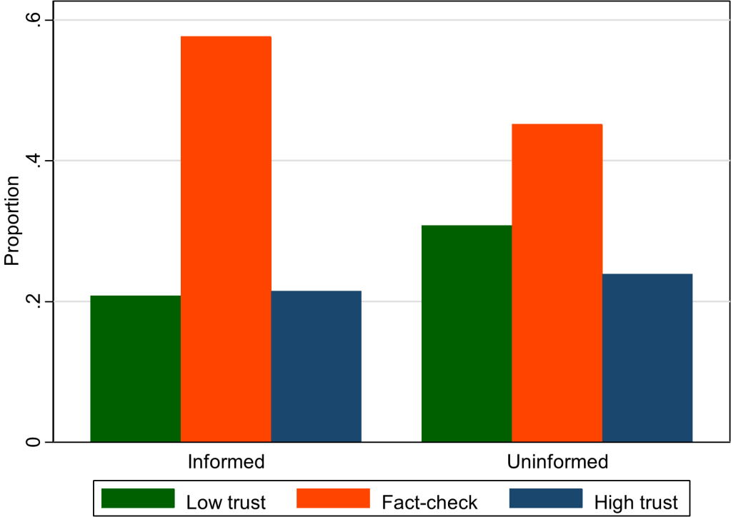
We presented information to participants in different ways. Sometimes we explicitly told them about authorship (informed treatment) and sometimes we asked them to guess about authorship (uninformed treatment).
This graph (figure 5 in our paper) shows that the overall rate of fact-checking increased when subjects were given more explicit information. Something about being told that a paragraph was written by a human might have aroused suspicion in our participants. (The kids today would say it is “sus.”) They became less confident in their own ability to rate accuracy and therefore more willing to pay for a fact-check. This effect is independent of whether participants trust humans more than AI.
We are thinking of fact-checking as often a good thing, in the context of our previous work on ChatGPT hallucinations. So, one policy implication is that certain types of labels can cause readers to think critically. For example, Twitter labels automated accounts so that readers know when content has been chosen or created by a bot.
Suggested Citation: Buchanan, Joy and Hickman, William, Do People Trust Humans More Than ChatGPT? (November 16, 2023). GMU Working Paper in Economics No. 23-38, Available at SSRN: https://ssrn.com/abstract=4635674
Citation: Buchanan, J., Hill, S., & Shapoval, O. (2024). ChatGPT Hallucinates Non-existent Citations: Evidence from Economics. The American Economist. 69(1), 80-87 https://doi.org/10.1177/05694345231218454
Blog followers will know that we reported this issue earlier with the free version of ChatGPT using GPT-3.5 (covered in the WSJ). We have updated this new article by running the same prompts through the paid version using GPT-4. Did the problems go away with the more powerful LLM?
The error rate went down slightly, but our two main results held up. It’s important that any fake citations at all are being presented as real. The proportion of nonexistent citations was over 30% with GPT-3.5, and it is over 20% with our trial of GPT-4 several months later. See figure 2 from our paper below for the average accuracy rates. The proportion of real citations is always under 90%. GPT-4, when asked about a very specific narrow topic, hallucinates almost half of the citations (57% are real for level 3, as shown in the graph).
The second result from our study is that the error rate of the LLM increases significantly when the prompt is more specific. If you ask GPT-4 about a niche topic for which there is less training data, then a higher proportion of the citations it produces are false. (This has been replicated in different domains, such as knowledge of geography.)
What does Joy Buchanan really think?: I expect that this problem with the fake citations will be solved quickly. It’s very brazen. When people understand this problem, they are shocked. Just… fake citations? Like… it printed out reference for papers that do not actually exist? Yes, it really did that. We were the only ones who quantified and reported it, but the phenomenon was noticed by millions of researchers around the world who experimented with ChatGPT in 2023. These errors are so easy to catch that I expect ChatGPT will clean up its own mess on this particular issue quickly. However, that does not mean that the more general issue of hallucinations is going away.
Not only can ChatGPT make mistakes, as any human worker can mess up, but it can make a different kind of mistake without meaning to. Hallucinations are not intentional lies (which is not to say that an LLM cannot lie). This paper will serve as bright clear evidence that GPT can hallucinate in ways that detract from the quality of the output or even pose safety concerns in some use cases. This generalizes far beyond academic citations. The error rate might decrease to the point where hallucinations are less of a problem than the errors that humans are prone to make; however, the errors made by LLMs will always be of a different quality than the errors made by a human. A human research assistant would not cite nonexistent citations. LLM doctors are going to make a type of mistake that would not be made by human doctors. We should be on the lookout for those mistakes.
ChatGPT is great for some of the inputs to research, but it is not as helpful for original scientific writing. As prolific writer Noah Smith says, “I still can’t use ChatGPT for writing, even with GPT-4, because the risk of inserting even a small number of fake facts… “
I still can't use ChatGPT for writing, even with GPT-4, because the risk of inserting even a small number of fake facts or bad interpretations into a blog post is unacceptable, meaning that it requires so much time to fact-check that it doesn't save effort.
Some economists love to write about sports because they love sports. Others love to write about sports because the data are so good compared to most other facets of the economy. What other industry constantly releases film of workers doing their jobs, and compiles and shares exhaustive statistics about worker performance?
To take an extreme example, suppose an average high-school athlete got thrown into a professional football or basketball game; a fan asked to evaluate them could probably figure out that they don’t belong there within minutes, or perhaps even just by glancing at them and seeing they are severely undersized. But what if an average high school coach were called up to coach at the professional level? How long would it take for a casual observer to realize they don’t belong? You might be able to observe them mismanaging games within a few weeks, but people criticize professional coaches for this all the time too; I think you couldn’t be sure until you see their record after a season or two. Even then it is much less certain than for a player- was their bad record due to their coaching, or were they just handed a bad roster to work with?
The sports economics literature seems to confirm my intuition that coaches are difficult to evaluate. This is especially true in football, where teams generally play fewer than 20 games in a season; a general rule of thumb in statistics is that you need at least 20 to 25 observations for statistical tests to start to work. This accords with general practice in the NFL, where it is considered poor form to fire a coach without giving him at least one full season. One recent article evaluating NFL coaches only tries to evaluate those with at least 3 seasons. If the article is to be believed, it wasn’t until 2020 that anyone published a statistical evaluation of NFL defensive coordinators, despite this being considered a vital position that is often paid over a million dollars a year:
A few months ago I looked at the richest and poorest MSAs in the US, including adjusting for the cost of living in each MSA. One big thing I found was that the list doesn’t change that much when you adjust for the cost of living: San Jose, San Francisco, Bridgeport (CT), Boston, and Seattle are still the highest income MSAs even after accounting for the fact that they are also high-cost-of-living places to live. The gap shrinks, but they are still in the lead.
But that was adjusting for all the factors in the cost of living. But what if we just looked at one important aspect of the cost of living: housing. And since the cost-of-living adjustments (BEA’s RPP) that I was using are from 2021, what if we tried to bring the data up as close to the present as possible? We know that housing prices have increased a lot since 2021, but also that the cost of borrowing has risen dramatically too. What would this show us about the cost of living for different MSAs?
A tool from the Harvard Joint Center for Housing Studies allows us to make some pretty up-to-date comparisons. Their interactive map shows data for the 179 largest MSAs (about half of the total MSAs in the US) on the median price of each home for the second quarter of 2023 and uses interest rates from that quarter to show the rough principal and interest cost (assuming a 3.5% down payment). Taxes and insurance costs for each MSA are also estimated.
Based on those assumptions, their tool provides the minimum income you would need to purchase a home in that area, assuming a 31% debt-to-income ratio for the mortgage. And the income levels needed vary quite widely across MSAs, from a low of $44,000 in Cumberland, Maryland, to a high of over $500,000 in San Jose, CA. That’s a huge difference.
Of course, we know that incomes also vary across MSAs. But they don’t vary that much. The JCHS tool doesn’t provide this data (though a JCHS map from 2017 did compare house prices to incomes), but we can look up median family income for each MSA from Census. Doing so we see that San Jose is indeed unaffordable based on the current (2022) median income, which is “only” about $170,000. A nice income compared to the national median, but only about 1/3 of the $500,000 you would need to afford a home in San Jose. Cumberland looks much better though: median family income is over $77,000 there, about 76% more than you would need to buy a home!
What if we did a similar calculation for all MSAs in the JCHS data? The following map is my attempt to do so. Sorry, but my graphics skills are not the best, so this map isn’t as pretty as it could be (I started with the JCHS map, and just shaded in the colors I wanted to use). But I think it conveys the general idea.
Green-shaded MSAs are the most affordable: places like Cumberland, Maryland, where median family income is well above (at least 20% above, my arbitrary threshold) the amount JCHS says you need to buy a home. There are 27 Green-shaded MSAs. Blue-shaded MSAs are affordable too, and median income is between 100% and 120% of the amount needed to afford a home on the JCHS standard. There are 41 of these, making 68 total MSAs out of these 179 that are affordable. Red-shaded MSAs are less than 100%, and thus unaffordable (though as I will discuss below, some are much closer to affordable than others).
A big piece of news in the investment world has been the passing of Charlie Munger on Nov 28 at age 99. He was vice chair of Berkshire Hathaway, and Warren Buffett’s right-hand man there.
Munger grew up in Omaha, Nebraska, which is Warren Buffett’s hometown as well. They met at a dinner party there in 1959, and hit it off with one another personally. Munger was a really smart guy. After joining the US Army Air Corps in1943, he scored highly on an intelligence test and was sent to study meteorology at Caltech. After the war he was accepted into Harvard Law School despite lacking a formal undergraduate degree, and graduated summa cum laude.
In his 50s, Munger lost his left eye after cataract surgery failed. A doctor warned he could lose his right eye too, so he began learning braille, but the condition improved.
He entered law practice, and eventually started his own firm, but he became more interested in investing. He racked up 19.8% annual returns investing on his own, between 1962 and 1975. Buffett convince Munger to give up law and join him as vice-chairman of Berkshire Hathaway in 1978.
Perhaps Buffett’s most famous investing saying is “It’s far better to buy a wonderful company at a fair price than a fair company at a wonderful price”. He credits this approach to Munger: “Charlie understood this early – I was a slow learner.” Before being influenced here by Munger, Buffett had been more inclined to buy very low-priced shares in mediocre companies.
Munger was heavily involved with Buffett’s decisions. “Berkshire Hathaway could not have been built to its present status without Charlie’s inspiration, wisdom and participation,” Buffett said following Munger’s death. That tribute is no overstatement: from the time Munger joined Berkshire Hathaway in 1978 till now, shares of the company soared 396,182% (i.e., $100 invested in Berkshire Hathaway in 1978 is worth $396,282 today). This performance dwarfs the 16,427% appreciation of the S&P 500 over the same time period. When he died, Munger was personally worth $2.6 billion.
The internet is rife with sites displaying memorable or useful quotes from Charlie Munger. For example, “I never allow myself to have an opinion on anything that I don’t know the other side’s argument better than they do”; and three rules for a career: “1) Don’t sell anything [to others] you wouldn’t buy yourself; 2) Don’t work for anyone you don’t respect and admire; and 3) Work only with people you enjoy.”
Some of these quote lists focus on sayings which provide guidance to individual investors, such as this from CNBC:
“I think you would understand any presentation using the word EBITDA, if every time you saw that word you just substituted the phrase, ‘bull—- earnings.’ ″
The 2003 Berkshire shareholder meeting was one of the many occasions Munger called out what he saw as shady accounting practices, in this case EBITDA — a measure of corporate profitability short for earnings before interest, taxes, depreciation and amortization.
In short, Munger felt that companies often highlighted convoluted profitability metrics to obscure the fact that they were severely indebted or producing very little cash.
“There are two kinds of businesses: The first earns 12%, and you can take it out at the end of the year. The second earns 12%, but all the excess cash must be reinvested — there’s never any cash,” Munger said at the same meeting. “It reminds me of the guy who looks at all of his equipment and says, ‘There’s all of my profit.’ We hate that kind of business.”
To invest like Munger and Buffett, don’t fall for the flashiest numbers in the firms’ investor presentations. Instead, dig into a company’s fundamentals in their totality. The more a company or an investment advisor tries to win you over with esoteric terms, the more skeptical you should likely be.
As Buffett put it in his 2008 letter to shareholders: “Beware of geeks bearing formulas.”
Munger’s Secret to Happiness
Out of all these witty and helpful quotes, I’ll conclude by zeroing in on what Charlie Munger thought was the single most important factor in achieving personal happiness. He said it a number of different ways:
A happy life is very simple. The first rule of a happy life is low expectations. That’s one you can easily arrange. And if you have unrealistic expectations, you’re going to be miserable all your life. I was good at having low expectations and that helped me. And also, when you [experience] reversals, if you just suck it in and cope, that helps if you don’t just stew yourself into a lot of misery.