Amazon Credit Card Rewards

I have a credit card that gives me rewards. I get a nice 5% cash-back on purchases from Amazon and a lower cash-back rate on other purchases. Sometimes, there are promotions that provide a rate of 10% or even 15%. But what are these rewards worth?

To simplify, there are two reward options:

Option 1 adds to my Amazon gift-card balance. It’s attractive. When I’m checking out at Amazon, it shows me my reward balance and it also shows me what the total cost of my purchase could be if I applied the gift card. It’s like they’re trying to pressure me to redeem my rewards in this particular way.

Option 2 is simply to transfer my rewards as a payment on my credit card or as a credit to my bank account (for the current purposes, they’re identical). Either way, the rewards translate to the same number of dollars.

Say that I spend $1,000 at Amazon. Whether I choose option 1 or 2 has value implications.

Option 1

The calculation is simple. If I spend $1,000 at amazon this month, then I can spend another $50 in gift card credits at Amazon next month. That’s the end. There are no more relevant cashflows. I used my credit card one month, and then was rewarded the next month. The only detail worth adding is the time value of money, which at 7% per year*, yields a present value of rewards at $49.72. Option 1 is nice in the moment. It’s so enticing to have a lower Amazon check-out balance due.

But you should never select Option 1.

Option 2

Continue reading →

Covid Evidence: Supply Vs Demand Shock

By the time most students exit undergrad, they get acquainted with the Aggregate Supply – Aggregate Demand model. I think that this model is so important that my Principles of Macro class spends twice the amount of time on it as on any other topic. The model is nice because it uses the familiar tools of Supply & Demand and throws a macro twist on them. Below is a graph of the short-run AS-AD model.

Quick primer: The AD curve increases to the right and decreases to the left. The Federal Reserve and Federal government can both affect AD by increasing or decreasing total spending in the economy. Economists differ on the circumstances in which one authority is more relevant than another.

The AS curve reflects inflation expectations, short-run productivity (intercept), and nominal rigidity (slope). If inflation expectations rise, then the AS curve shifts up vertically. If there is transitory decline in productivity, then it shifts up vertically and left horizontally.

Nominal rigidity refers to the total spending elasticity of the quantity produced. In laymen’s terms, nominal rigidity describes how production changes when there is a short-run increase in total spending. The figure above displays 3 possible SR-AS’s. AS0 reflects that firms will simply produce more when there is greater spending and they will not raise their prices. AS2 reflects that producers mostly raise prices and increase output only somewhat. AS1 is an intermediate case. One of the things that determines nominal rigidity is how accurate the inflation expectations are. The more accurate the inflation expectations, the more vertical the SR-AS curve appears.*

The AS-AD model has many of the typical S&D features. The initial equilibrium is the intersection between the original AS and AD curves. There is a price and quantity implication when one of the curves move. An increase in AD results in some combination of higher prices and greater output – depending on nominal rigidities. An increase in the SR-AS curve results in some combination of lower prices and higher output – depending on the slope of aggregate demand.

Of course, the real world is complicated – sometimes multiple shocks occur and multiple curves move simultaneously. If that is the case, then we can simply say which curve ‘moved more’. We should also expect that the long-run productive capacity of the economy increased over the past two years, say due to technological improvements, such that the new equilibrium output is several percentage points to the right. We can’t observe the AD and AS curves directly, but we can observe their results.

The big questions are:

  1. What happened during and after the 2020 recession?
  2. Was there more than one shock?
  3. When did any shocks occur?

Below is a graph of real consumption and consumption prices as a percent of the business cycle peak in February prior to the recession (See this post that I did last week exploring the real side only). What can we tell from this figure?

Continue reading →

This Time was Way Different

The financial crisis recession that started in late 2007 was very different from the 2020 pandemic recession. Even now, 15 years later, we don’t all agree on the causes of the 2007 recession. Maybe it was due to the housing crisis, maybe due to the policy of allowing NGDP to fall, or maybe due to financial contagion. I watched Vernon Smith give a lecture in 2012 in which he explained that it was a housing crisis. Scott Sumner believes that a housing sectoral decline would have occurred, and that the economy-wide deep recession and subsequent slow recovery was caused by poor monetary policy.

Everyone agrees, however, that the 2007 recession was fundamentally different from the 2020 recession. The latter, many believe, reflected a supply shock or a technology shock. Performing social activities, including work, in close proximity to others became much less safe. As a result, we traded off productivity for safety.

The policy responses to each of the two were also different. In 2020, monetary policy was far more targeted in its interventions and the fiscal stimulus was much bigger. I’ll save the policy response differences for another post. In this post, I want to display a few graphs that broadly reflect the speed and magnitude of the recoveries. Because the recessions had different causes, I use broad measures that are applicable to both.

Continue reading →

Russia, The US, and Crude Data

Overall, I’ve been disappointed with the reporting on the US embargo against Russian oil. The AP reported that the US imports 8% of Russia’s crude oil exports. But then they and other outlets list a litany of other figures without any context for relative magnitudes. Let’s shine some more light on the crude oil data.*

First, the 8% figure is correct – or, at least it was correct as of December of 2021. The below figure charts the last 7 years of total Russian crude oil exports, US imports of Russian crude oil, and the proportion that US imports compose.  That 8% figure is by no means representative of recent history. The average US proportion in 2015-2018 was 7.8%. But the US share as since risen in level and volatility. Since 2019, the US imports compose an average of 11.9% of all Russian crude oil exports.

As an exogenous shock, the import ban on Russian crude oil might have a substantial impact on Russian exports. However, many of the world’s oil importers were already refusing Russian crude. The US ban may not have a large independent effect on Russian sales and may be a case of congress endorsing a policy that’s already in place voluntarily.

Continue reading →

Two Decades of Real Estate Data

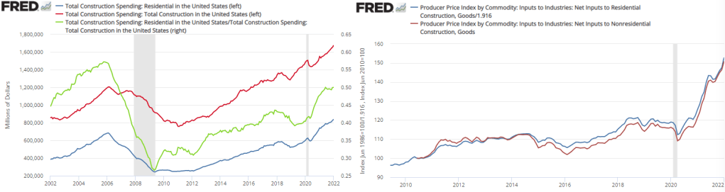
Total spending on real estate construction has been rising since 2011. By 2016 it had reached its previous 2006 peak. However, total spending on *residential* real estate construction didn’t reach its previous 2006 peak until November of 2020. The graph below also includes the proportion of residential construction spending (Green). It has been rising since 2009. In and of itself, nothing is good or bad about this figure. We might be spending less on non-residential construction because we are getting better at using less land per unit of good or service produced. Or, it could be that our real investment in future production is falling relative to our current residential consumption.  Regardless, the share of residential construction hasn’t been at this level since 2003.

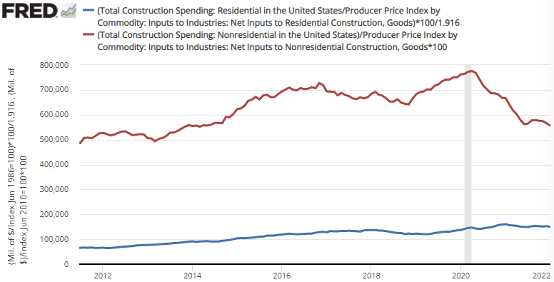
Importantly, the difference in spending has not been driven by different construction costs. Both residential and non-residential construction costs have moved in tandem since 2010. Therefore, the rise in residential construction spending is not merely nominal – a greater proportion of resources are being consumed by residential construction. Indeed, real residential construction is up about 25% from 2019. The figure below illustrates real residential and nonresidential construction.

That figure requires a double-take.

Continue reading →

Inflation Empirics

Way back in the late 1970s and early 80s, Kydland and Prescott proposed rational expectations theory. This line of research arose, in part, because the Phillips curve ceased to describe reality well. Amid increasing inflation, people began to anticipate higher prices to a relatively correct degree when making labor, supply chain, and pricing decisions. Kydland and Prescott argued that individuals understand the rules of the game or how the world works – at least on average.

An increase in the money supply would increase total national spending, and increase demand for goods. However, firms also experienced increasing revenues and demanded more inputs such as commodities, capital, and intermediate goods. Because there were no greater productivity earlier in the supply chain, price roses. Firms began to understand that greater demand would eventually find its way to causing greater costs. Therefore, firms began raising prices before the cost of resources rose, increasing their willingness to pay for inputs and, ironically, hastening the increase in input prices. As a result, increases in the money supply began having substantial short-run price effects and negligible output effects.

However, assuming that people understand the rules of our economic system and ‘how the world works’ is hard to swallow. It is not at all clear that the typical economist understands monetary theory, much less clear that the typical person has a good understanding. Fortunately, another theory of expectations can help carry some of the load and achieve similar results.

Adaptive Expectations

Continue reading →

Asymmetric Liability, Common Law, & Urbanization

Tort law is interesting. You can argue that someone harmed you, and you can cite almost no legislation in the process. Torte law in the US uses case law – the precedent set by previous rulings in the context of social norms. But, what cases did the early cases cite? They also cited earlier cases and social norms, though we may no longer have a record. The beauty of tort law it allows for changing relative costs in prudence and negligence.

Can you imagine a legislature attempting to codify the appropriate amount of neglect by, say, a painter? The standards would quickly go out of date. The relative cost of resources including labor, communications, materials, and the price differences among competitors of differing quality all change over time. Multiply these factors by 20 and then again by the number of occupations and regions in a country. You will quickly see that legislating the appropriate degree of prudence and neglect through congress is a fool’s errand. The challenge is too complicated and the world changes too quickly. In fact, attempting to legislate definitions for neglect and prudence could even backfire and result in regulatory arbitrage, which occurs when firms comply with de jur rules while avoiding them de facto.*

Externalizing Costs

Continue reading →

Mises’s Bureaucracy, a Recap

My favorite two economists are Ludwig Von Mises and Milton Friedman. They might consider one another from very different schools of thought, though there is reason to think that they are not so different. As an undergraduate student, I liked them both, but I became more empirics-minded in graduate school and as a young assistant professor.

As I progressed through graduate school and conducted empirical research, my opinions and policy prescriptions changed and were refined from what they once were. In graduate school, I didn’t study Austrian Economics, though it was certainly in the water at George Mason University. Recently, as an assistant professor with a few years under my belt, I picked up Bureaucracy (1944) and read it as a matter of leisure.

One word:

Continue reading →

Teaching Price Controls (Poorly)

Economics textbooks differ in their treatment of price controls. None of them does a great job, in my opinion. The reason is mostly due to the purpose of textbooks. Despite what you might suspect, most undergraduate textbooks are not used primarily to give students an understanding of the world. They are often used as a bound list of things to know and to create easy test questions. If a textbook has to change the assumptions of a model too much from what the balance of the chapter assumes, then the book fails to make clear what students are supposed to know for the test.

I think that this is the most charitable reason for books’ poor treatment of price controls – even graduate level books. The less charitable reasons include sloppy exposition due to author ignorance or an over-reliance on math. I honestly would have trouble believing these less charitable reasons.

I picked up 5 microeconomics text books and the below graph is typical of how they treat a price ceiling.

The books say that the price ceiling is perfectly enforced. They identify producer surplus (PS) as area C and consumer surplus (CS) as areas A & B. There are very good reasons to differ with these welfare conclusions.

Problem #1

Continue reading →

Fences, Schools, Dryer Lint, & Shower Levers

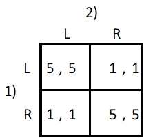
In game theory, coordination games reflects the benefits of everyone settling on the same rules. Settling on the same rules can avoid a conflict and destructive competition. For example, some rules may be arbitrary, such as on which side of the road we’ll all drive. It doesn’t much matter whether a country’s vehicles drive along the right or left side of the street. As long as everyone is in the same lane, we overwhelmingly benefit from our coordination. The matrix below describes the game.

The above game reflects that whether we agree to drive on the left or on the right is trivial and that the important detail is that we agree on what the rule is. Rules like this are arbitrary. No amount of cost benefit analysis changes the answer. Other coordination rules are seemingly arbitrary, but do have different welfare implications. For example, according to English common law, a farmer was entitled to prohibit a herdsman’s flock from trampling his crops even if the farmland had no fence. Herdsmen were responsible for corralling their flocks or paying damages if they grazed on the farm. With lots of nearby farms, total welfare was higher with a rule of cultivation rights rather than grazing rights.

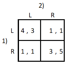
But the property rights could have been assigned to the herdsman instead. The law could have said that the sheep were free to graze with impunity and that the onus was on the farmer to build fences in order to keep the sheep at bay. In a world where there are a lot of farmers who are very nearby to one another, a small flock of sheep can do a lot of damage. And so, the cost-benefit analysis prescribes that herdsmen bear the cost of restricting the flock rather than the farmer. The matrix that describes this circumstance is below.

The above matrix reflects that agreeing on any rule is better than no rule at all. And, the rule that is selected has societal welfare implications. Choosing the ‘wrong’ rule means that we could get stuck in a rut of lower payoffs because coordinating a change in the rules is hard.

Schools

Another way in which the specific rule can be important is by whether it instantiates or works contrary to pre-existing incentives. Before compulsory schooling laws were passed, US states already had very high school attendance rates. Most parents sent their kids to school because it was a good investment. The ages at which children should be required to attend is largely, though not entirely, arbitrary. And wouldn’t you know it, most states applied their compulsory schooling legislation to the age groups for which the vast majority of children were already attending school. Enforcing a law against the natural incentives of human capital investment would have been more costly. The particular ages of compulsory schooling had different welfare implications due to the differing costs of enforcement.

Dryer Lint

Continue reading →