I watched the Chapman Economic Forecast Update for 2023 live on June 22 (you can watch the whole thing free here). Go to their website for free videos and links. They have an excellent track record for being correct.
This time, Dr. Jim Doti believes we are headed for a recession by the third quarter of 2023 or at least what he conservatively calls a “slowdown”. He hates to make dramatic predictions or deliver bad news, but he saw the inflation brewing back in 2021, and I remember him correctly predicting what was to come.
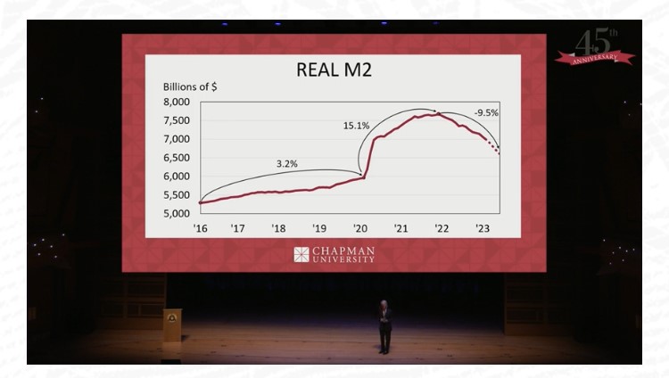
For one thing, the dramatic growth in the money supply at the beginning of the pandemic has been corrected into a sharp contraction of the money supply.
People have been joking about how the recession isn’t happening.
The middle segment of the forecast, which I recommend watching, is about investing. Fadel Lawandy cautions that stocks are not a good bet right now, with a likely recession looming.
The third segment is focused on the economy of California. I didn’t finish that part, since I don’t live there anymore.
My wife makes this great chili recipe. She called me yesterday as I departed from work and asked me to grab some beer on the way home (it’s the secret ingredient in case you need to zhuzh up your version). So, I went to my local overpriced grocer. The options were dire. All the good 6-packs were way overpriced. The 12-packs, though a lower unit price, weren’t much better.
Luckily a ‘fine’ beer was on sale at an OK price ($17.49 for 12). Not what I wanted, but fine. I did self check-out and noticed that the price that I paid was not the sale price – by a healthy $2. A ‘fine’ beer at an ok price is one thing. But a ‘fine’ beer at a ‘great’ beer price is no bueno. After check-out, I made a b-line for the beer aisle in order to double check myself. Me making a mistake is often a good first approximation. But nuts – I was mischarged.
I took a photo of the ‘correct’ price and headed to the customer service desk.
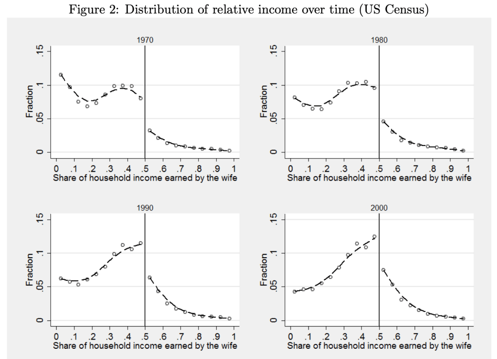
As we have gone through our education and training and changed jobs, my wife and I have been in every sort of relative income situation, with each one sometimes vastly or slightly out-earning the other. Currently she slightly out-earns me, which I thought was unusual, as I remembered this graph from Bertrand, Kamenica and Pan in the QJE 2015:
The paper argues that the big jump down at 50% is driven by gender norms:
this pattern is best explained by gender identity norms, which induce an aversion to a situation where the wife earns more than her husband. We present evidence that this aversion also impacts marriage formation, the wife’s labor force participation, the wife’s income conditional on working, marriage satisfaction, likelihood of divorce, and the division of home production. Within marriage markets, when a randomly chosen woman becomes more likely to earn more than a randomly chosen man, marriage rates decline. In couples where the wife’s potential income is likely to exceed the husband’s, the wife is less likely to be in the labor force and earns less than her potential if she does work. In couples where the wife earns more than the husband, the wife spends more time on household chores; moreover, those couples are less satisfied with their marriage and are more likely to divorce.
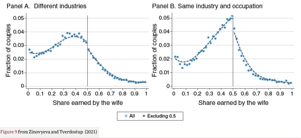
But when I went to look up the paper to show my wife the figures, I found that the effect it highlights may no longer be so large. Natalia Zinovyeva and Maryna Tverdostup show in their 2021 AEJ paper that the jump down in wives’ income at 50% is quite small, and is largely driven by couples who have the same industry and occupation:
They created the figure above using SIPP/SSA/IRS Completed Gold Standard Files, 1990–2004. I’d be interested in an analysis with more recent data. Much of their paper uses more detailed Finnish data to test the mechanism for the remaining jump down at 50%. They conclude that gender norms are not a major driver of the discontinuity:
We argue that the discontinuity to the right of 0.5 can emerge if some couples tend toward earnings equalization or convergence. To test this hypothesis, we exploit the rich employer-employee–linked data from Finland. We find overwhelming support in favor of the idea that the discontinuity is caused by earnings equalization in self-employed couples and earnings convergence among spouses working together. We show that the discontinuity is not generated by selective couple formation or separation and it arises only among self-employed and coworking couples, who account for 15 percent of the population.
Self-employed couples are responsible for most observations with spouses reporting identical earnings. When couples start being self-employed, both sides of the distribution tend to equalize earnings, perhaps because earnings equalization helps couples to reduce income tax payments, facilitate accounting, or avoid unnecessary within-family negotiations. Large spikes emerge not only at 0.5 but also at other round shares signaling the prevalence of ad hoc rules for entrepreneurial income sharing in couples. Self-employment is associated with a fall of household earnings below the level predicted by individuals’ predetermined characteristics, but this drop is mainly due to a decrease in male earnings, with women being relatively better off.
In the case of couples who work together in the same firm, there is a compression of the earnings distribution toward 0.5 both on the right and on the left of 0.5. As a result, there is an increase both in the share of couples where men slightly outearn their wives and in the share of couples where women slightly outearn their husbands. Since the former group is larger, earnings compression leads to a detection of a discontinuity.
So, concerns about relative earnings aren’t causing trouble for women in the labor market. But do they cause trouble at home? Perhaps yes, but if so its not in a gendered way and not driven by the 50% threshold:
Separation rates do not exhibit any discontinuity around the 0.5 threshold of relative earnings. Instead, the relationship between the probability of separation and the relative earnings distribution exhibits a U-shape, with higher separation rates among couples with large earnings differentials either in favor of the husband or in favor of the wife.
62 weeks. That’s how long the median male worker would need to work in a year to support a family in 2022, according to the calculations of Oren Cass for the American Compass Cost-of-Thriving Index released this year. Not only is 62 weeks longer than the baseline year of 1985 (when it took about 40 weeks, according to COTI), but there is a big problem: there aren’t 62 weeks in year. It is, by this calculation, impossible for a single male earner to support a family.
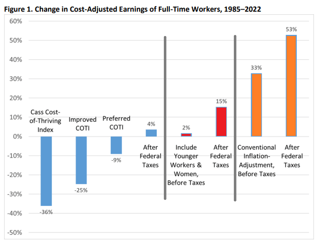
Is this true? In our new AEI paper, Scott Winship and I strongly disagree. First, we challenge the 62-week figure. With a few reasonable corrections to Cass’ COTI, we show that it is indeed possible for a median male earner to support a family. It takes 42 weeks, not 62 as reported in COTI.
But wait, there’s more. Much more. In our paper, we provide a range of reasonable estimates for how the cost of thriving has changed since 1985. In the COTI calculation, the standard of living for a single-earner family has fallen by 36 percent since 1985. In our most optimistic estimate, the standard of living has risen by 53 percent. The chart below summarizes our various alternative versions of COTI. How do we get such radically different results? Is this all a numbers game?
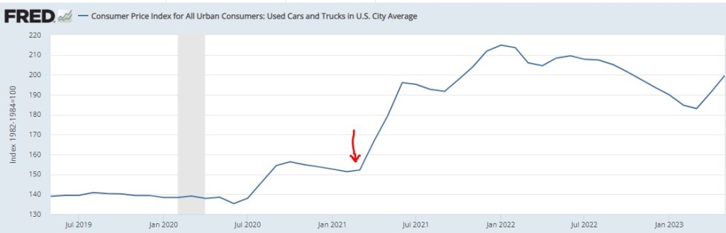
I write about various topics, usually with at least some loose connection to economics. Sometimes these are fairly macro issues, other times there are specific, actionable observations. For instance, back in March of 2021, we inferred from the critical shortages of semiconductors that car manufacturing would be severely crimped, likely leading to big price increases in cars. Our post “Chip Shortages Shutting Down Auto Assembly Lines; Buy Your Car Now Or Else” came out just in time (red arrow below) to alert the readership here:
But now, a price increase of more ubiquitous import looms. Most of us were not in the market for cars in March of 2021, but some 81% of us eat chocolate, with the average American consuming about 9.5 pounds a year. Indeed, 50% “cannot live without it every day.”
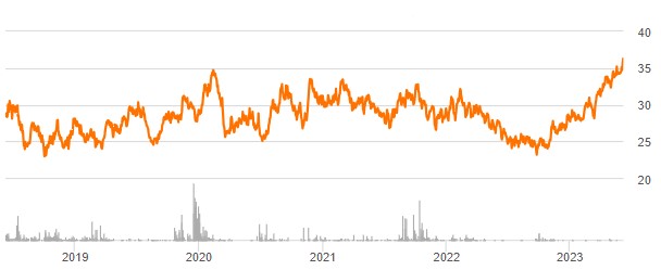
And so, it is with a heavy heart that I bring warning of a rise in the price of chocolate. Back in pandemic lockdown, I was bored and speculated a few bucks in cocoa futures, as tracked by the NIB exchange traded fund. My shares went up, and then down, and I sold out to limit losses (which was a good move at the time), and moved onto other investments.
Imagine my surprise when I randomly checked on NIB this week and saw the price ramp-up in the past few months:
A quick internet search led to a CNBC article which confirmed my worst fears:
“The cocoa market has experienced a remarkable surge in prices … This season marks the second consecutive deficit, with cocoa ending stocks expected to dwindle to unusually low levels,” S&P Global Commodity Insights’ Principal Research Analyst Sergey Chetvertakov told CNBC in an email.
The price of cocoa will feed into the price of consumer chocolate products, especially dark chocolate which has more actual cocoa content. And the price of sweets generally will rise on the back of sugar prices, which stand at 11-year highs, driven again largely by weather.
There is still time to stock up ahead of the hoarders…
I’ll keep it brief today. The best golfers in the world are usually in the running, but who wins depends on who flips heads on the most coins i.e. who makes the most putts. Putting is a skill to be sure, but there is enough chaos in the green that randomness has a heavy say in who wins. Skill can wholly dominate when the differences between the best and everyone else is greater than multiple standard deviations of a coldly binomial distribution.
The greatest record in golf is not who won the most tournaments, but Tiger Woods making 142 consecutive cuts after the first two days of tournaments. He was so much better than everyone else that even when every coin flip went against him he was still in the top half of the leaderboard. The greatest record in tennis is Roger Federer making 23 consecutive semifinals in major tournaments. The greatest record in the NBA may be Lebron James reaching the NBA finals 8 times in a row, including with some Cleveland teams exceedingly thin on talent. The home run record is nice, but Barry Bonds greatest achievement may be his reaching base 61% of at-bats in 2004. 61%! To put that in context, the leader last year reached base 42.5% of the time.
The mark of true excellence is when repeated competition reveals a gap from their opposition so great that even the cruel left tail of randomness can rarely overcome it.
I’m writing an article about fast-fashion, so I’m reading Fashionopolis by Dana Thomas.
This paragraph is from the intro chapter:
Since the invention of the mechanical loom nearly two and a half centuries ago, fashion has been a dirty, unscrupulous business that has exploited humans and Earth alike to harvest bountiful profits. Slavery, child labor, and prison labor have all been integral parts of the supply chain at one time or another – including today. On occasion, society righted the wrongs, through legislation or labor union pressure. But trade deals, globalization, and greed have undercut those good works.
She invokes religion with “good works.” Thomas and I are of different opinions concerning globalization and “greed” and legislation. My instinct is to rip this paragraph apart. Has legislation never been motivated by greed? Has globalization not improved the lives of children? Has the mechanical loom not improved the lives of women who used to spend hours spinning and weaving by hand?
I am also reading pastor Tim Keller’s biography right now, so I’m having a What Would TK Do moment.
With his gifts (smart, funny, articulate…), Keller could have made a fortune by taking a side. He could have picked the Right or the Left. He could have expertly appealed to a Side, convincing them that they were good-smart and the Other is evil-stupid. Instead, Keller relentlessly stayed in the center. One of his books is actually called Center Church.
There have been a lot of popular papers in the past decade or so that make use of textual analysis. A fun one is “The Mainstreaming of Marx” by Magness & Makovi. They use Google Ngram to analyze the popularity of people mentioned in books and determine when Karl Marx became popular. “Measuring Economic Policy Uncertainty” by Baker, Bloom, & Davis is one of my favorites. They use set theory to detect terms in newspapers that denote economic policy uncertainty. In this post, I’m just going to describe practical differences between the two data sources and how the interpretations differ.
Ngram
Ngram measures takes a term and measures how popular that term is in its corpus of book text, which is about 6% of all books ever written (in English, anyway). Because popularity is expressed as a percent, we can make direct popularity level comparisons among words. For example: “Cafe” & “Coffee Shop”. In the figure below, we can see that the word “cafe” was more popular in books until very recently.
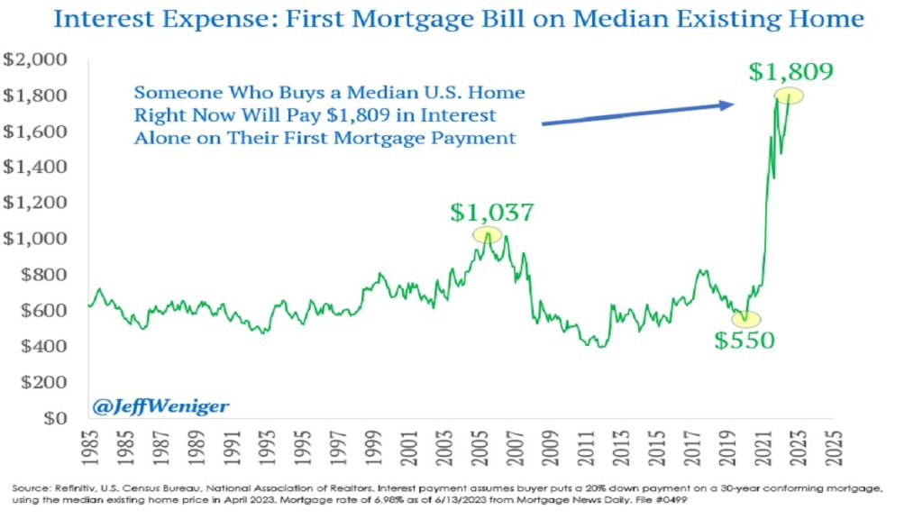
The Federal Reserve has been increasing interest rates at the fastest pace since the 1980’s, from near-zero rates in March of last year to over 5% today. This has led to rapid slowdowns in interest-rate sensitive sectors like housing, cars, and startups. Because most people finance their home buying, higher interest rates mean higher monthly payments for a house at a given price. Since many people were already buying houses near the highest monthly payment banks would allow them to, higher interest rates mean they need to buy cheaper houses or just stay out of the market and rent. This is especially true as the interest expense on mortgages has tripled in two years:
You’d think this would be bad news for homebuilders, and for most of 2022 markets agreed: homebuilder stocks fell 36% from the beginning of 2022 to September 2022 after the Fed started raising rates in March. But homebuilder stocks have recovered since September, with some major names like D.R. Horton and Lennar hitting all time highs. Why?
I bought homebuilder stocks in January but I have to say even I wasn’t expecting such a fast recovery (if I had, I would have bought a lot more). I was buying because they were cheap on a price to earnings basis and temporarily out of fashion; I love stocks that are priced like they’re in a secular decline to bankruptcy when its clear they are actually just having a bad cycle and will recover when it turns. But I thought I’d have to wait years for falling interest rates and a recovering housing market for this to happen. Instead these are up 20-100% in 6 months. Why?
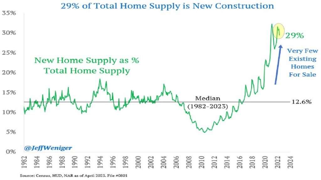
The big thing I missed was that high interest rates have hit their competition harder, reducing supply as well as demand. Who is the competition for homebuilders? Existing homeowners. Homeowners with the “golden handcuffs” of a 3% mortgage who don’t want to move if it means switching to a 7% mortgage. I’m seeing this personally in Rhode Island- I’d kind of like a house with a bigger yard on a quieter street, but there are only 5 houses for sale in my whole school district. Between that and interest rates, we’re staying put. But for people who really need to move, new homes are making up a record proportion of the available inventory:
This situation seems likely to persist for at least months, and possibly years. The Fed paused its rate hikes yesterday for the first time since last March, but indicated that more hikes may lie ahead. I’m tempted to take the win and sell homebuilder stocks, but they still have price to earnings ratios under 10, and the “golden handcuffs” on their competition seem likely to stay on for at least another year.
On summer vacation, I recently visited Mount Rushmore. It’s amazing structure, and the story of its construction is as impressive as the monument itself. Much of the story you learn when visiting is the story of its creation. As an economist, of course seeing the following display with wage data got me very excited:
While the sign says that laborers made 30 cents per hour, searching online it appears that 50 cents was more common. More skilled workers, such as assistant sculptors, made $1.50 per hour. These were, as the sign says, “good wages” for that time. In the economy generally, production workers made around 50 cents per hour our as well around that time period, and most of the construction of Rushmore was during the Depression (some of the workers were WPA funded), so having any job, much less one that paid pre-Depression wages, was certainly a good one.
How does this compare to wages today? This is always a tricky question, as I have documented on this blog several times before, but the most straight forward approach (and good first approximation) is a simple CPI inflation adjustment. Using 1929 as the baseline year, when construction was in full swing, 30 cents an hour is roughly $5 today, 50 cents per hour is close to $9, and $1.50 would be about $26.50. That doesn’t sound too bad!
The best comparison I like to use is BLS’s average hourly earnings for private production and non-supervisory workers. Averages aren’t perfect, but this measure excludes management occupations that will be distorting the average. In May 2023, that wage was $28.75 per hour. So the average worker today earns 3-6 times as much per hour as these “good paying jobs” in the late 1920s and the Depression. And, as the Rushmore signage notes, these jobs were seasonal. Their off-season jobs probably paid even less.
The wage of the assistant sculptor does compare well with average wages today, but that pay was unusual for the time and was likely a highly skilled worker. The only record I can find of anyone making that much at Rushmore was Lincoln Borglum, the son of the main sculptor Gutzon Borglum. Lincoln oversaw the completion of the project after Gutzon’s death, and it was only in later years on the project that his pay was increased to $1.50 per hour.
For the typical laborer on Rushmore, having a good job was indeed good to have, but the wages pale in comparison to a typical worker today.