As you may have heard, there have been a few bank failures in the US in the past week. This has led ordinary people to start refreshing their memory about exactly what “deposit insurance” is and what it means for them. It has also led regulators, politicians, and economists to start refreshing their memory about the social purpose of deposit insurance, which is to stabilize the banking system. There are lots of aspects of the bank failures and deposit insurance to consider, but I think we can all agree that when ordinary people are thinking about this topic, bad things are going on.
While I can’t find a systematic survey of economists on this topic, my guess is that most economists would agree with the statement “on balance, deposit insurance promotes stability in the financial system.”
But there is a minority view, and one with (in my opinion) considerable historical support. Deposit insurance could potentially be destabilizing, since it has the potential (like any form of insurance) to create moral hazard. By lowering the cost of making mistakes, we would expect more mistakes. The cost need not be lowered all the way to zero for moral hazard to be a problem (bank owners still have some skin in the game), but the cost is certainly lower. These problems may be even more of a threat to the financial system than other areas of life covered by insurance.
That’s the theory. What’s the evidence?
My favorite paper on this topic is a 1990 article by Charles Calomiris called “Is Deposit Insurance Necessary? A Historical Perspective.” Not only does it conclude that deposit insurance isn’t necessary, but even more: it may be destabilizing. (You can also read a version of the article intended for a more general audience that Calomiris wrote for the Chicago Fed.)
Much ink has been spilled making cross-country comparisons since the start of the COVID-19 pandemic. I have made a few of these, such as a comparison of GDP declines and COVID death rates among about three dozen countries in late 2021. I also made a similar comparison of G-7 countries in early 2022. But all such comparisons are tricky to interpret if we want to know why these differences exist between countries, which surely ultimately we would like to know. I tried to stress in those blog posts that I was just trying to visualize the effects, not make any claims about causation.
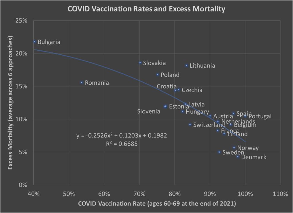
Here’s one more chart which I think is a very useful visualization, and it may give us some hint at causation. The following scatterplot shows COVID vaccination rates and excess mortality for a selection of European countries (more detail below on these measures and the countries selected):
The selection of countries is based on data availability. For vaccination rates, I chose to use the rate for ages 60-69 at the end of 2021. Ages 60-69 is somewhat arbitrary, but I wanted a rate for an elderly age group that was somewhat widely available. There is no standard source for an international organization that published these age-specific vaccine rates (that I’m aware of), but Our World in Data has done an excellent job of compiling comparable data that is available.
Note: I’m using the data on at least one dose of the vaccine. OWID also has it available by full vaccine series, and by booster, but first dose seemed like a reasonable approach to me. Also, I could have used different age groups, such as 70-79 or 80+, but once you get to those age groups the data gets weird because you have a lot of countries over 100%, probably due to both challenging denominator calculations and just general challenges with collecting data on vaccination rates. By using 60-69, only one country in my sample (Portugal) is over 100%, and I just code them as 100%. Using the end of 2021, rather than the most current data, is a bit arbitrary too, but I wanted to capture how well early vaccination efforts went, though ultimately it probably wouldn’t have mattered much.
Also: dropping the outliers of Bulgaria and Romania doesn’t change things much. The second-degree best fit polynomial still has an R2 over 0.60 (for those unfamiliar with these statistics, that means about 60% of the variation is “explained” in a correlational sense).
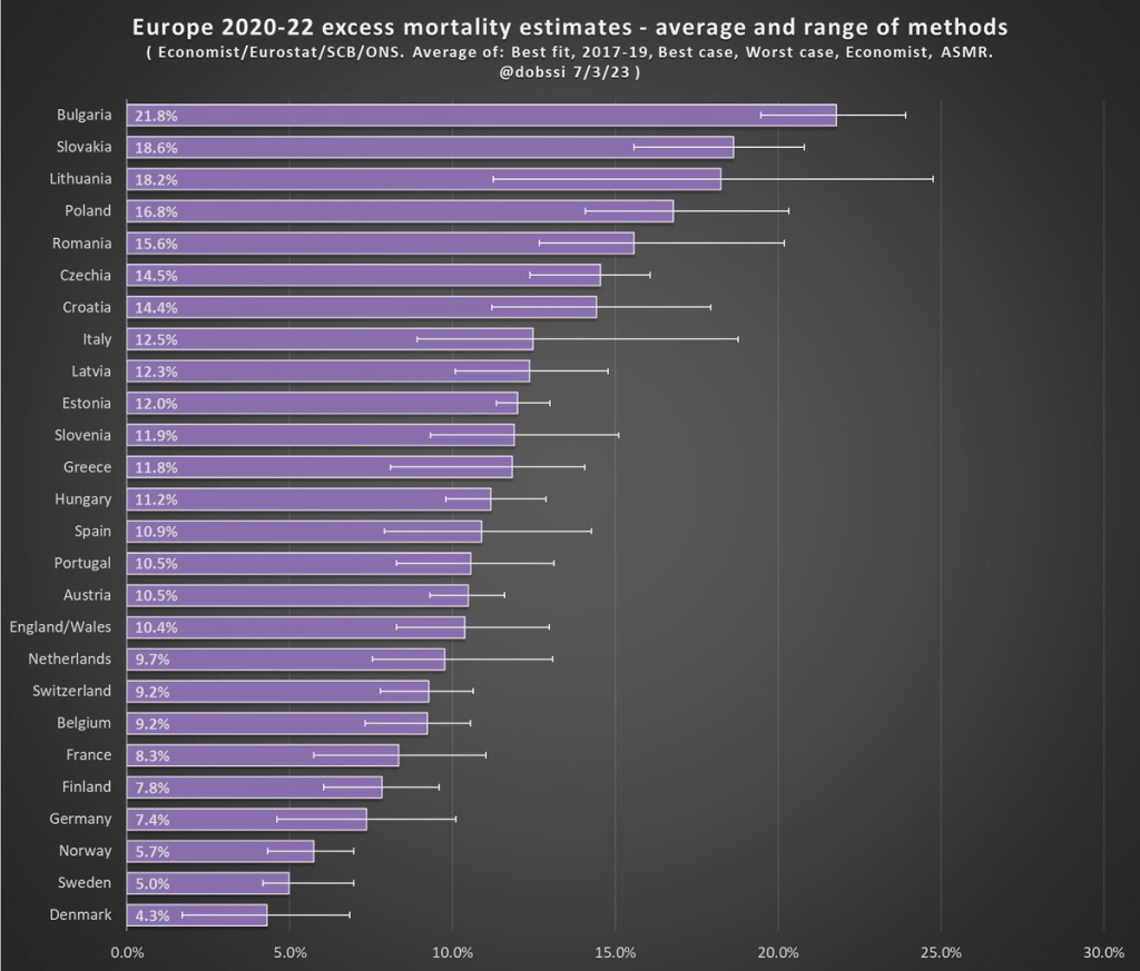
The excess mortality measure I use comes from the following chart. In fact, this entire post is inspired by the fact that this chart and others similar to it have been shared frequently on social media.
The chart comes from a Tweet thread by Paul Collyer. The whole thread is worth reading, but this chart is the key and summary of the thread. What he has done is shown the average and range of a variety of ways of calculating excess mortality. Read his thread for all the details, but the basic issues are what baseline to use (2015-2019 or 2017-2019? A case can be made for both), how to do the age-standardized mortality, and other issues. I won’t make a claim as to which method is best, but averaging across them seems like a fine approach to me.
For the y-axis in my chart, I just used the average for each country from Collyer’s chart. There are 34 countries in his chart, but in the OWID age-specific vaccination rates, only 22 countries were available the overlapped with his group. Unfortunately, this means we drop major countries like Italy, Spain, the UK, and Germany, but you work with the data you have.
For many sharing this and similar chart (such as charts with just one of those methods), the surprising (or not surprising) result to them is that Sweden comes out with almost the lowest excess mortality rate. Some approaches even put Sweden as the very lowest. Sweden!
Why is Sweden so important? Sweden has been probably the most debated country (especially by people not living in the country in question) in the COVID pandemic conversation. In short, Sweden took a less restrictive (some might say much less restrictive) approach to the pandemic. This debate was probably the most fevered in mid-to-late 2020, when some were even claiming that the pandemic was over in Sweden (it wasn’t). The extent to which Sweden took a radically different approach is somewhat overstated, especially in relation to other Nordic countries. And as is clear in both charts above, the Nordic countries all did relatively very well on excess mortality.
The bottom line from my first chart is that what really matters for a country’s overall excess mortality during the pandemic is how well they vaccinated their population. There seems to be a lot of interest on social media to rehash the debates about whether lockdowns (and lighter restrictions) or masks worked in 2020. But what really mattered was 2021, and vaccines were key. A scatterplot isn’t the last word on this (we should control for lots of other things), but it does suggest that a big part of the picture is vaccines (you can see this in scatterplots of US states too). It’s frustrating that many of those wanting to rehash the 2020 debates to “prove” masks don’t work, or whatever, either ignore vaccines or have bought into varying degrees of anti-vaccination theories. It’s completely possible that lockdowns don’t pass a cost/benefit test, but that vaccines also work very well (this has always been my position).
Why did Sweden have such great relative performance on excess mortality? Vaccines are almost certainly the most important factor among many that matter to a much smaller degree.
What About the US?
Note: for those wondering about the US, we don’t have the vaccination rate for ages 60-69 that I can find. Collyer also didn’t include the US in his analysis, it was only Europe. So, for both reasons, I didn’t include them in this post. The CDC does report first-dose vaccinations for ages 65+ in the US, though they top-code states at 95%. As of the end of 2021, here are the states that were below 95%: Mississippi, Louisiana, Tennessee, West Virginia, Indiana, Ohio, Wyoming, Georgia, Arkansas, Idaho, Alabama, Montana, Alaska, Missouri, Texas, Michigan, and Kentucky. These states generally have very high age-adjusted COVID death rates. Ideally we would use age-adjusted excess mortality for US states, but in the US that is horribly confounded by the rise in overdoses, homicides, car accidents, and other causes that are independent of vaccination rates (though they may be related to 2020 COVID policies — this is still a matter of huge debate).
There are many papers with titles in the style of “The Economics of X” with X covering a wide variety of topics, some deadly serious (“Economics of Suicide“) and others more trivial or unintentionally hilarious (“The Economics of Sleep and Boredom” comes to mind). There is a related genre of papers on “The Political Economy of Y,” once again with papers that are both serious and occasionally silly (or sometimes deadly serious papers with silly-sounding titles, such as “The Political Economy of Coffee, Dictatorship, and Genocide“).
But perhaps the best paper of this sort is a 1974 article on the Journal of Political Economy by Alan Blinder, titled “The Economics of Brushing Teeth.” It is, as you might guess, a paper that is somewhat tongue-in-cheek (tongue-in-teeth?), but the paper carefully follows the formal style you would expect from a JPE paper in 1974. I recommend reading the paper in full, and I can assure you that it is not at all like pulling teeth. But if you prefer not to look a gift horse in the mouth, here are a few favorite parts.
The paper is, of course, full of tooth-related puns, even in the footnotes, such as this acknowledgment: “I wish to thank my dentist for filling in some important gaps in the analysis.”
There are also plenty of jokes about human capital theory, jokes that only an economist could love, such as: “The basic assumption is common to all human capital theory: that individuals seek to maximize their incomes. It follows immediately that each individual does whatever amount of toothbrushing will maximize his income.”
Another section manages to poke fun at both sociologists and economists. In reference to a fake paper (no, there is no Journal of Dental Sociology), Blinder chastises the fake sociologist for misattributing a change in brushing patterns (assistant professors brush more) to advancing hygiene standards over time. No! It must be about maximizing income: “To a human capital theorist, of course, this pattern is exactly what would be expected from the higher wages received in the higher professorial ranks, and from the fact that younger professors, looking for promotions, cannot afford to have bad breath.”
And what good is a paper without a formal model of teeth brushing? This is the kind of model that many young economists cut their teeth on in graduate school.
The minimum wage is one of the most studied topics in economics, and also something that is frequently discussed on this blog from many different angles. For someone that isn’t an expert in this area, it can be hard to keep track of all the most recent, cutting-edge research on the topic.
Here’s a brand-new paper in the literature with an important finding: raising the minimum wage increases crime. Specifically, in “The Unintended Effects of Minimum Wage Increases on Crime” the authors find that 16-to-24-year-olds commit more property crimes after a minimum wage increase. For every 1% increase in the minimum wage, there is a 0.2% increase in property crime. That implies a doubling the minimum wage would increase property crimes for this age group by 20%. Here’s a figure from the paper showing this increase in crime:
What is the mechanism by which the rising minimum wage increases crime? Here the authors move into examining one of the central questions of the empirical minimum wage debate: the labor market. The authors do find evidence that employment decreases for this same age group following an increase in the minimum wage. Again, a figure from the paper:
The results in this paper add one more element to the cost-benefit calculus of the minimum wage. But I think the results are also interesting because they seem to point in the opposite direction of a paper co-authored by fellow EWED blogger Mike Makowsky. His paper “The Minimum Wage, EITC, and Criminal Recidivism” found that increasing the minimum wage made it less likely that former prisoners would commit another crime. I would be interested to hear Mike’s thoughts on this paper!
Tyler Cowen is skeptical about the possibility of a pure land-value tax, even though it has many theoretical benefits. In particular, Cowen points to a host of what we might call “Public Choice NIMBY” issues. In the real world, the same political forces that drive all of the current urban planning issues would either prevent it from being implemented at all, or prevent it from actually being implemented the way Henry George would have wanted.
I grant all these objections, but I do note that there have been multiple YIMBY successes in recent years, particularly in California where NIMBY forces are probably the strongest in the country. Still, if Cowen is mostly correct, are there any real-world options that offer some of the benefits of a LVT? In short, the main benefits are that the deadweight loss of the tax is very small, and that land is more likely to be used for its highest-valued use (which in many cases will mean more density, though this intersects with zoning policy).
Yes. For the clearest example, look to Pennsylvania. Cities are allowed to implement what is called a “split-rate property tax.” It does not only tax land, as a pure LVT would do, but instead taxes land at a higher rate than improvements. A ratio around 5:1 is typical (meaning land is taxed at 5 times the rate of improvements), though some cities have been as high as 26:1.
Black families are the poorest major racial or ethnic group in the US. With a median income of $59,541, a Black family only has about 59 percent of the income of a White, Non-Hispanic family. That’s the same proportion, 59 percent, as was true in 1972, the earliest date that we have comparable data. (For most of the data in this post, I will be using Table F-23 from the Census Bureau’s Historical Income Tables.) That’s almost 50 years with no closing of the racial gap in total money income for families.
Of course, what this also means is that family incomes of both Black and Whites grew at the same rate from 1972 to 2021. They both are about 50 percent larger than in 1972, and that’s after accounting for inflation (using the CPI-U-RS). As a first point of optimism, this very much goes against the typical narrative of income stagnation since the early 1970s.
To be sure, some of this growth is because families have more earners today, but even so: they have a lot more income. Having two earners does mean that you must spend more on some consumption categories, such as daycare when kids are young, possibly more on dining out or prepared meals. But even with those additional expenses, these families will have significantly more disposable income than their 1970s counterparts.
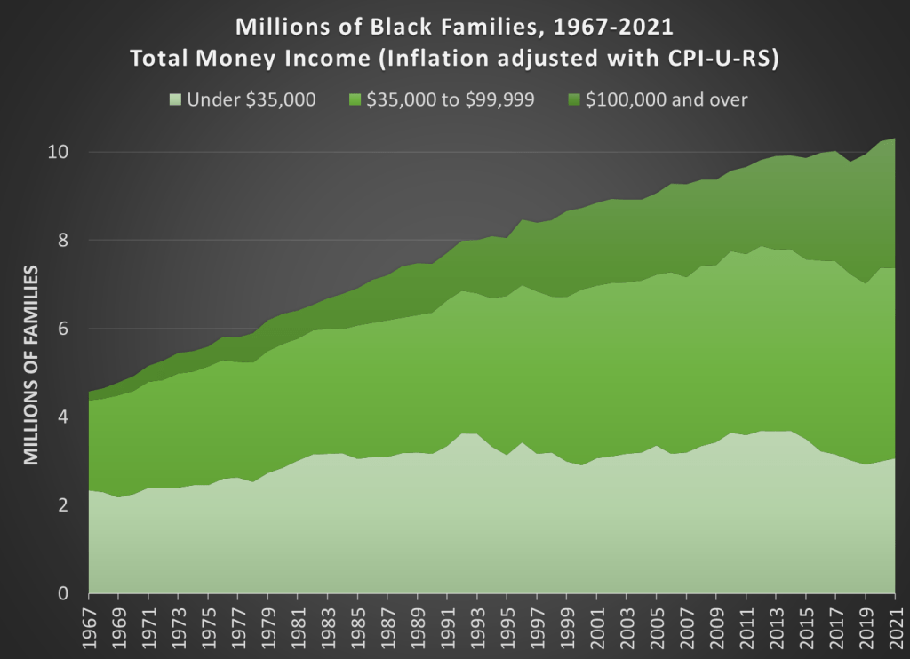
There is an ever more optimistic fact that we need to point out for Black families today: there are many, many more rich Black families today than in 1972. There are more rich families in absolute terms and as a proportion of the total. Here is the basic data from the Census Bureau (it goes back to 1967, the earliest date available for Blacks).
How well have countries recovered from the declines in the pandemic? It’s actually a bit difficult to answer that question, because it depends on how you measure it. Even if we agree that GDP is the best measure, how do we measure recovery? One possibility is to simply ask whether the country has exceeded its pre-pandemic GDP level. Exactly which quarter to use as the baseline is debatable, but here is a chart that Joseph Politano made for G7 countries using the 3rd quarter of 2019 as the baseline.
But we know that absent the pandemic, most countries would have continued growing (absent a recession for some other reason), so just getting back to pre-pandemic levels isn’t necessarily a full recovery. But how much growth should we have expected? It’s a hard question, but here’s a chart along those lines from the Washington Post, using the CBO’s measure of “potential GDP” as what growth might have looked like.
Using either of these approaches, it appears that the US has recovered pretty well, although it would be nice to have a comparison across countries using the same approach as the Washington Post chart does. While there is no consistent measure similar to CBO’s potential GDP figure for all countries, a simple approach is to project growth forward using the average pre-pandemic growth rate. I have done so for a number of countries, using the average growth rate from 2017-2019. In the following charts, the blue line is actual GDP levels, and the orange line is projecting the 2017-2019 growth rate forward. Sorry that I can’t easily fit all these into one chart, so here come the charts!
Last week I wrote about the challenges of counting deaths. But surely in economics, we can count better, especially when it comes to something concrete like the number of people working. Right?
Maybe not. If you follow the economic data regularly, you’ll know that once per month, the Bureau of Labor Statistics releases data on the employment situation of the nation’s economy. And if you are familiar with this report, you will probably know that it is based on two separate surveys, one of businesses and one of households. And furthermore, it gives us two separate measures of employment, the number of people working for pay.
Joseph Politano has been tracking the employment situation reports, and he writes that the two measures of employment have “completely diverged since March of [2022], with the establishment survey showing payroll growth of nearly 2.7 million and the household survey showing employment growth of 12,000.” The surveys are tracking the labor market differently, so it’s not surprising that they won’t be exactly the same (they rarely are), but this sort of discrepancy is huge. Even accounting for most of the differences between the surveys, there is still a gap of about 2 million jobs.
Today, the BLS released yet another measure of employment, this one comes from the Business Employment Dynamics series. The BED is not released as quickly as the data in the employment situation report — the BED data released today is for the 2nd quarter of last year. But that’s because this data is much more comprehensive, and it’s actually the same data underlying the employment measure from businesses in the monthly employment report (it comes from unemployment insurance records, which covers most of the workforce).
What did the BED find for the 2nd quarter of 2022? A net loss of 287,000 jobs. The BED is only looking at private-sector jobs, and it is also seasonally adjusted to smooth out normal quarterly fluctuations. If we look back at the monthly data on employment, what did it look like in the 2nd quarter of 2022? Using the seasonally adjusted, private-sector jobs number to match the BED, it showed a gain of 1,045,000 jobs. In other words, we have a discrepancy of 1.3 million jobs in a single quarter. This is huge.
Perhaps some of this could be attributed to different seasonal adjustment factors, but even using the unadjusted data there is still a gap: 3,089,000 jobs added in the monthly payroll survey (private sector only), but only a net gain of 2,432,000 private-sector jobs in the BED data. That discrepancy is smaller, but it is still a difference of over 600,000 jobs. Note here that there was job growth in the second quarter in the BED measure, just not enough job growth that on a seasonally adjusted basis that it showed net growth. Another way to think of this: there is almost always growth in the 2nd quarter, but we expected it to be a bit stronger than this data shows.
If you aren’t confused enough yet, BLS produces yet another measure of employment, called the Quarterly Census of Employment and Wages. Really this is the broadest measure of jobs and is using the same underlying data as the BED and monthly nonfarm jobs in the business survey. But like the BED, it is also released with a significant lag. What does it show? A gain of 2,338,000 jobs in the 2nd quarter of last year (this includes public sector employment too). That number isn’t seasonally adjusted and compares with the CES (monthly nonfarm employment) number of 2,702,000, a discrepancy of 364,000 jobs (note: the CES will later be revised and benchmarked with the QCEW data).
What can we learn from all these different estimates of jobs? And which is right? The short answer to the second question is: they are all right, but measuring different things. The big takeaway is that there was indeed job growth in the 2nd quarter of 2022 (even the household survey shows job growth), but based on more complete data the monthly business survey probably overstated job growth, and it may have actually been pretty weak job growth compared to what we would normally expect in that quarter in the private sector (but of course, we aren’t in normal times).
How many people died in the US from heart diseases in 2019? The answer is harder than it might seem to pin down. Using a broad definition, such as “major cardiovascular diseases,” and including any deaths where this was listed on the death certificate, the number for 2019 is an astonishing 1.56 million deaths, according to the CDC. That number is astonishing because there were 2.85 million deaths in total in the US, so over half of deaths involved the heart or circulatory system, at least in some way that was important enough for a doctor to list it on the death certificate.
However, if you Google “heart disease deaths US 2019,” you get only 659,041 deaths. The source? Once again, the CDC! So, what’s going on here? To get to the smaller number, the CDC narrows the definition in two ways. First, instead of all “major cardiovascular diseases,” they limit it to diseases that are specifically about the heart. For example, cerebrovascular deaths (deaths involving blood flow in the brain) are not including in the lower CDC total. This first limitation gets us down to 1.28 million.
But the bigger reduction is when they limit the count to the underlying cause of death, “the disease or injury that initiated the train of morbid events leading directly to death, or the circumstances of the accident or violence which produced the fatal injury,” as opposed to other contributing causes. That’s how we cut the total in half from 1.28 million to 659,041 deaths.
We could further limit this to “Atherosclerotic heart disease,” a subset of heart disease deaths, but the largest single cause of deaths in the coding system that the CDC uses. There were 163,502 deaths of this kind in 2019, if you use the underlying cause of death only. But if we expand it to any listing of this disease on the death certificate, it doubles to 321,812 deaths. And now three categories of death are slightly larger in this “multiple cause of death” query, including a catch-all “Cardiac arrest, unspecified” category with 352,010 deaths in 2019.
So, what’s the right number? What’s the point of all this discussion? Here’s my question to you: did you ever hear of a debate about whether we were “overcounting” heart disease deaths in 2019? I don’t think I’ve ever heard of it. Probably there were occasional debates among the experts in this area, but never among the general public.
COVID-19 is different. The allegation of “overcounting” COVID deaths began almost right away in 2020, with prominent people claiming that the numbers being reported are basically useless because, for example, a fatal motorcycle death was briefly included in COVID death totals in Florida (people are still using this example!).
A more serious critique of COVID death counting was in a recent op-ed in the Washington Post. The argument here is serious and sober, and not trying to push a particular viewpoint as far as I can tell (contrast this with people pushing the motorcycle death story). Yet still the op-ed is almost totally lacking in data, especially on COVID deaths (there is some data on COVID hospitalizations).
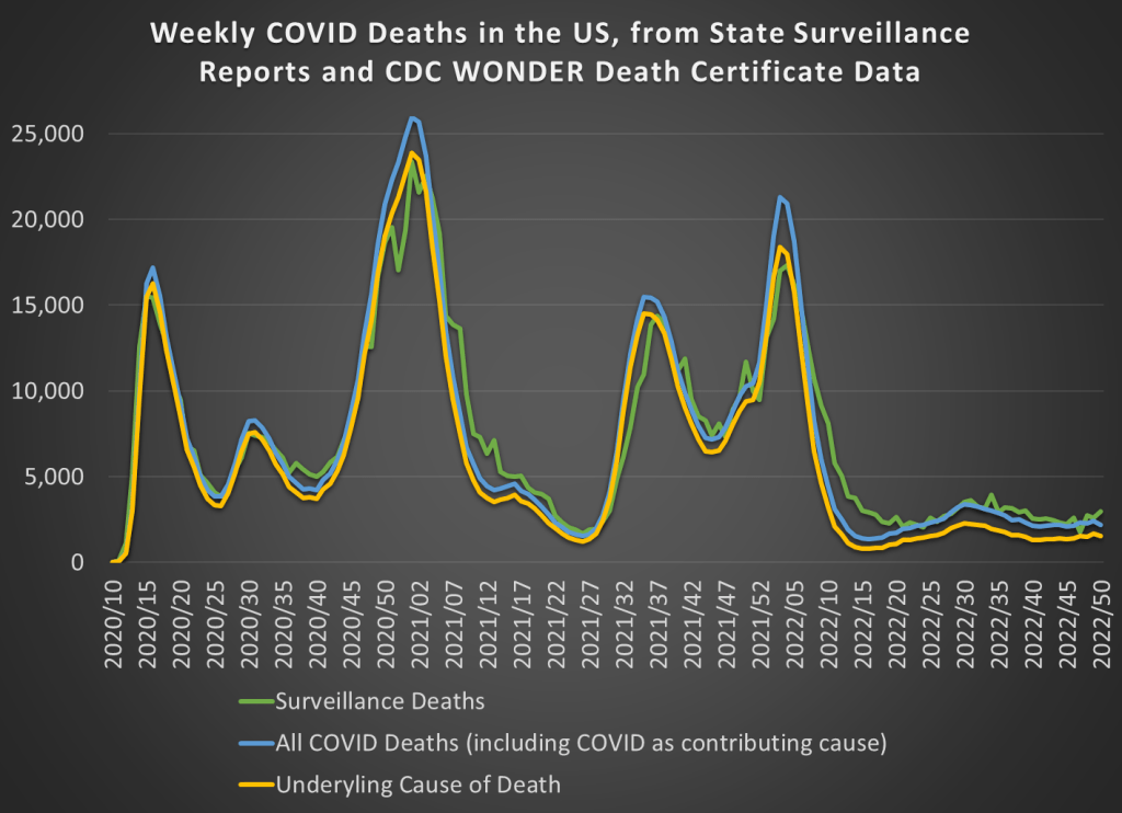
But most of the data she is asking for in the op-ed is readily available. While we don’t have death totals for all individuals that tested positive for COVID-19 at some point, we do have the following data available on a weekly basis. First, we have the “surveillance data” on deaths that was released by states and aggregated by the CDC. These were “the numbers” that you probably saw constantly discussed, sometimes daily, in the media during the height of the pandemic waves. The second and third sources of COVID death data are similar to the heart disease data I discussed above, from the CDC WONDER database, separated by whether COVID was the underlying cause or whether it was one among several contributing causes (whether it was underlying or not).
Those three measures of COVID deaths are displayed in this chart:
If you look at the long-run trends in labor markets, one of the most obvious changes is the decline in working hours. The chart from Our World in Data shows the long-run trend for some countries going back to 1870.
Hours of work declined in the US by 43% since 1870. In some countries like Germany, they fell a lot more (59%). But the decline was substantial across the board. One thing to notice in the chart above is that for the very recent years, the US is somewhat of an outlier in two ways. First, there hasn’t been much further decline after about the mid-20th century. Second, average hours of work in the US are quite a bit higher than many of developed countries (though similar to Australia).
But the labor market in the US (and in other countries) is in a very unusual spot at the present moment after the pandemic. So what has happened really recently. Many economists are looking into this question of hours and other questions about the labor market, and a new working paper titled “Where Are the Workers? From Great Resignation to Quiet Quitting” presents a lot of fascinating data about the current state of work in the US. The paper is short (just 14 pages) and readable for non-experts, so I encourage you to read it all yourself.
Here is one table and one chart from the paper that I will highlight, which shows that hours of work have been falling, but in a very specific set of workers: those who work lots of hours, and those with high incomes. For workers at the high end of hours worked, the 90th percentile, they have dropped from 50 hours to 45 hours of work per week just from 2019 to 2022. But workers at the median? Unchanged at 40 hours per week. (The data comes from the CPS.)
The figure below is only for male workers, and it shows a similar decline in hours worked for those at the high end of the earnings distribution. For those at the bottom, hours of work at mostly unchanged.