The United States is a uniquely violent country among high-income democracies. And by the best available data on homicides, the US has always been more violent. Homicides are useful to look at because we generally have the best data on these (murders are the most likely crime to be reported) and it’s the most serious of all violent crimes.
Just how much more violent is the US than other high-income democracies? As measured by the homicide rate, about 6-7 times as violent. We can see this first by comparing the US to several European countries (and a few groupings of similar countries).
Let me make a few things clear about this chart. First, this is data for homicides, which are typically defined as interpersonal violence. Thus, it excludes deaths on the battlefield, genocides, acts of terrorism (generally speaking), and other deaths of this nature. That’s how it is defined. If we plotted a chart of battlefield deaths, it would look quite different, but there’s not much good reason to combine these different forms of violent death.
On the specifics of the chart, prior to 1990 these data are averages from multiple observations over multi-year timespans (generally 25 or 50 years). The data on European countries comes from a paper by Eisner on long-term crime trends (Table 1). The countries chosen are from this paper, as are the years chosen. Remember that historical data is always imperfect, but these are some of the best estimates available. For the US, I used Figure 5 from this paper by Tcherni-Buzzeo, and did my best to make the timeframes comparable to the Eisner data. The data are not perfect, but I think they are about as close as we can get to long-run comparisons. For the data from 1990 forward, I use the IHME Global Burden of Disease study, and the death rates from interpersonal violence (to match Eisner, I average across grouped countries).
When we average across all the European countries in the first chart and compare the US to Europe, we can see that the US has always been more violent, though the 20th century onwards does seem to show even more violence in the US relative to Europe. (These charts are slightly different from some that I posted on Twitter recently, especially the pre-1990 data as I tried to more carefully use the same periods for the averages — still only take this a rough guide).
And what is the main form by which this violence is carried out? In the US, it is undeniably clear: firearms. Between 1999 and 2020, there were almost 400,000 homicides in the US (using CDC data). Over 275,000 of these, or about 70%, were carried out with firearms. The next largest category is murder with a knife or other sharp object, with about 10% of murders. And homicides have become even more gun-focused in recent years: about 80% of murders in 2020-21 were committed with guns.
So, there’s the data. But the important social scientific question is: Can we do anything about it? Are there any public policies, either about guns or other things, that will reduce gun violence? Could restrictions on gun use actually increase homicides, since no doubt guns are also used defensively?
In July of 1992, the Barenaked Ladies released their debut studio album Gordon, which included one of their most popular songs: “If I Had $1000000.” Considering all the inflation we’ve had recently, you know that $1 million doesn’t buy as much as it did in 1992, but how much less? As measured by the Consumer Price Index in the US, prices have roughly doubled since 1992, meaning you would need about $2 million to buy the same amount of stuff as in 1992.
(Note: the Barenaked Ladies are Canadian, and prices in Canada haven’t quite doubled since 1992, but this song was included on early demo tapes in 1988 and 1989 released in Canada, and prices have roughly doubled there since then.)
So the value of a dollar that you held since 1992 has lost roughly half of its purchasing power. That’s bad. But how bad is it? What’s the normal US experience for how long it takes for prices to double?
It turns out that even with the recent huge run-up in inflation, we just lived through the lowest period of inflation for anyone alive today.
In previous blog posts, I’ve used the Simpsons as an example of a typical family to use for historical comparisons. In a post on mortgage payments, I found that it’s slightly easier to make a mortgage payment on Homer’s salary than in the early 1990s. In a post on taxes, I showed that the Simpsons now pay a much lower average tax rate than they did in the 1990s (guess all those tax cuts didn’t just go to the rich!).
Now, the Simpsons and economics are back at the front of the discourse about standards of living. The 33rd season finale of the show is all about whether the middle class can get by economically these days. And Planet Money’s “The Indicator” podcast (great program!) has a podcast about the show, which is a follow-up to a similar podcast last year called “Are The Simpsons Still Middle Class?” (apparently part of the influence for the recent Simpsons episode).
In that podcast from last year, they say “Tuition has more than doubled. Health care costs have more than doubled. I believe housing costs have more than doubled.” And they follow-up, for good measure with “Even after adjusting for inflation, college tuition has more than doubled since ‘The Simpsons’ started.”
Since we’ve already looked at housing costs for Homer, let’s look at the potential college costs for Bart. I’m going to assume Lisa will be fine, probably getting a free-ride (and a hot plate!) to one of the Seven Sisters or maybe even Harvard. But if Bart wants to go to college, the Simpsons will probably be paying out of pocket.
An important factor to consider when looking at college prices is not just the “sticker price,” or the published price, but to also look at what is known as the “net price.” The net price takes into account the average amount of aid that a student receives. This is important to consider at any time, but especially for data in more recent years since discounting has become a major part of the college pricing landscape. For example, at private colleges the average discount is now over 50%, with some colleges essentially giving some discount to 100% of students (in other words, at some colleges no one actually pays the sticker price). Discounting at public colleges isn’t quite as out-of-control as private colleges, but it’s still a major part of college pricing.
And no doubt Bart Simpson would be going to a traditional public, four-year college. Probably Springfield University, just like his old man (though Homer attended as an adult), located right in their town of Springfield. So what has happened to tuition prices since the early 1990s.
One of the best publications on college prices is the College Board’s annual report “Trends in College Pricing.” The report is broken down by type of college, it shows what factors (tuition, housing, etc.) make up the typical cost of college, and even shows differences across US states. Importantly, they include that “net tuition and fees” number, and they’ve been doing so since their 2003 report. That 2003 report even calculated the net figures back to the 1992-93 school year, perfect for an example of the early Simpsons (“Homer Goes to College” aired in 1993).
In the 1992-93 academic year, the average net tuition and fees, plus room and board for public four-year colleges in the US was $4,620 (from Figure 7, adjusted back to nominal dollars). In the 2020-21 academic year, the same figure was $15,050 (from Figure CP-9). Adjusted for inflation, that’s roughly a doubling (slightly less, but in the ballpark) since the early 1990s, just as Planet Money stated.
But let’s compare the cost of college to Homer’s income. In 1992, the median male with a high school education, working full-time earned $26,699, meaning that the cost of college would be 17.3% of his income that year. In 2020, the median male with a high school education, working full-time earned $49,661, meaning that the cost of college would be 30.3% of his income.
By this measure, college clearly has become much more expensive when compared to a Homer Simpson-type salary, and 30% of your income is a very hard pill to swallow (though the 17% in 1992 wasn’t a picnic either). But here’s one other factor to consider. The College Board data also allows us to look only at net tuition and fees, rather than also including the cost of room and board. Remember, Springfield University is located in Springfield, and Bart has a perfectly fine room at the house on Evergreen Terrace. While living on campus is certainly a big part of the college experience, and no one would probably love that experience more than Bart Simpson, many students today do choose to live with their parents while attending college (or at least live off-campus, where housing is often cheaper).
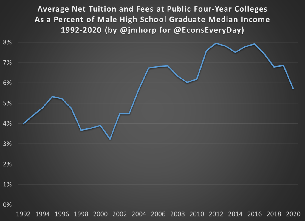
If we just look at net tuition and fees (not room and board), in 1992-93 the average cost at public four-year colleges was about $1,065 (in nominal dollars). That’s about 4% of Homer’s annual income. Much more reasonable! In 2020-21, that same figure was $2,880 (once again, in nominal dollars), or just under 6% of annual income. That’s certainly more than 4%, but not exactly the kind of expense that would break the budget if planned for.
I want to repeat that number again: $2,880. That was the average cost of tuition and fees at an in-state, four-year, public college in the US in 2020-21, after accounting for grants and aid. I suspect this number is much, much lower than most would guess.
The chart below does the same calculation for all the years I could find (1992-2020) using archived versions of the College Board’s report. I’ll admit the data isn’t perfect, as later reports sometimes have different numbers than earlier reports, but it’s probably the best we can do if we want a consistent time series. There does seem to be a break happening in the early 2000s, when college suddenly did get more expensive relative to a high school graduate’s income, though in the past 15 years it’s been pretty flat.
We should keep in mind that if Bart were to take out the maximum federal student loan amount of $9,000 as a dependent student in his first year at Springfield University, he is primarily borrowing money to pay for his housing and food, not his education.
In 1993, the premium for getting a college degree was about 54%, with the median male college grad earning about $41,400 and the equivalent high school grad earning about $26,800 (data from Table P-24). In 2021, that premium had risen to about 64%, with the median male college grad earning $81,300 compared with his high school counterpart earning about $49,700.
I’m ignoring all sorts of important questions here about what is causing the difference in pay. Is it signaling, human capital, something else, or some combination of all these? Yes. But regardless of your preferred explanation for the college wage premium, there’s pretty solid evidence of a sheepskin effect.
Putting It All Together
I’ve now explored taxes, housing, and college education prices using a family like the Simpsons. But what if we put it all together? How are high school graduates doing?
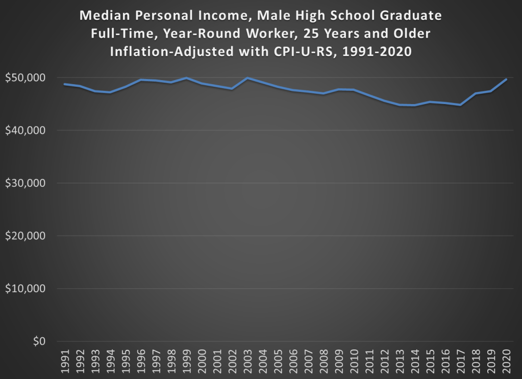
The best way to do this is probably the simple chart you’ve been thinking of all along: median income adjusted for inflation. Some things have gotten cheaper (housing, TVs), some more expensive (college, probably healthcare), but to get a sense of the total effect, we need to adjust for all prices. The chart below is that calculation, using Census data on median earnings for full-time, year-round workers, male high school graduates aged 25 and older. The data starts in 1991. You can get some earlier estimates from different data series, but if we want a consistent series 1991 is the best we can do.
And from the chart we see that real incomes of male high school graduates are… pretty flat. That’s not good, but let’s contextualize. First, claims that it’s harder for these workers to make ends meet aren’t true. It’s roughly no easier, but also no harder. Definitely wage stagnation, but also not “falling behind.”
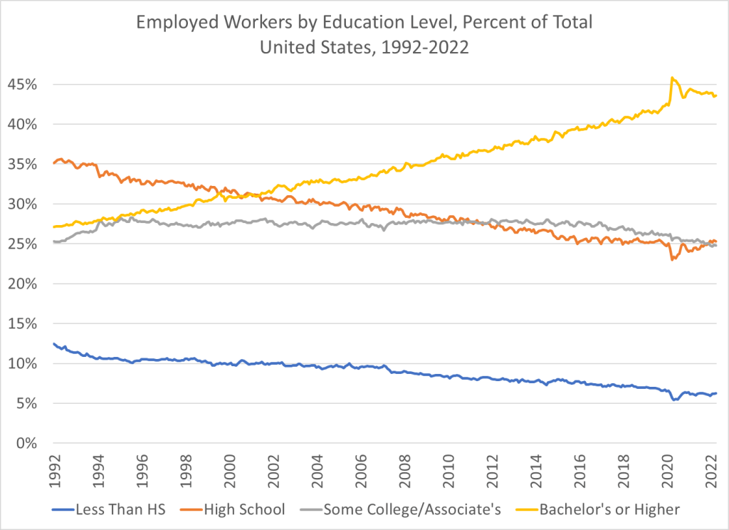
And also, high school graduates are a shrinking part of the workforce in the United States. You probably already knew this. But it wasn’t until after the year 2000 that college grads became the largest category of workers in the US. In the early 1990s, high school graduates (folks like Homer) were by far the largest single category of workers. Now, it’s by far college graduates, and those with some college or a 2-year degree are roughly equal in size to high school graudates. So, while the income stagnation we see for high school grads is not good, it’s affecting a shrinking portion of workers in the US.
While we know that COVID primarily affects the elderly, the mortality and other effects on the non-elderly aren’t trivial. I have explored this in several past posts, such as this November 2021 post on Americans in their 30s and 40s. But now we have more complete (though not fully complete) mortality data for 2021, so it’s worth revisiting the question of COVID and the non-elderly again.
For this post, I will primarily focus on the 12-month period from November 2020 through October 2021. While data is available past October 2021 on mortality for most causes, data classified by “intent” (suicides, homicides, traffic accidents, and importantly drug overdoses) is only fully current in the CDC WONDER data through October 2021. This timeframe also conveniently encompasses both the Winter 2020/21 wave and the Delta wave of COVID (though not yet the Omicron wave, which was quite deadly).
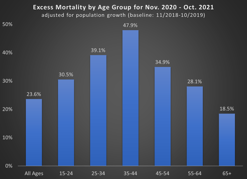
First, let’s look at excess mortality using standard age groups. For this calculation, I use the period November 2018 through October 2019 as the baseline. The chart shows the increase in all-cause deaths in percentage terms. It is also adjusted for population growth, though for most age groups this was +/- 1% (the 65+ group was 3% larger than 2 years prior).
A few things jump out here. First notice the massive increase in mortality for the 35-44 age group (much more on this later). Almost 50% more deaths! To put that in raw numbers, deaths increased from about 82,000 to 122,000 for the 35-44 age group, and population growth was only about 1%. And while that is the largest increase, there were huge increases for every age group that includes adults.
Also notice that the 65+ age group certainly saw an increase, but it is the smallest increase among adults! Of course, in raw numbers the 65+ age group had the most excess deaths: about 450,000 of the 680,000 excess deaths during this time period. But since the elderly die at such high rates in every year, the increase was as large in percentage terms.
One related fact that doesn’t show up in the chart: while there were about 680,000 excess deaths during this time frame in the US in total, there were only about 480,000 deaths where COVID-19 was listed as the underlying cause of death. That means we have about 200,000 additional deaths in this 12-month time period to account for, or a 24% increase (population growth overall was only 0.4%).
That’s a lot of other, non-COVID deaths! What were those deaths? Let’s dig into the data.
The latest CPI inflation report didn’t have a huge surprise in the headline number, with 8.3% being very similar to last month. But with the two most recent months of data, we can now see something very unfortunate in the data: cumulative inflation during the pandemic as measured by the CPI-U (11.6%) has now almost matched average wage growth (12.0%), as measured by the average wage for all private workers. I start in January 2020 for the pre-pandemic baseline.
What this means is that inflation-adjusted wages in the US are no greater than they were before the pandemic. They are almost identical to what they were in February 2020 (just 2 cents greater). But as regular readers will know, the CPI-U isn’t the only measure of inflation, and there’s good reason to believe it’s not the best. One alternative is the Personal Consumption Expenditures price index. Cumulative inflation for the PCE is slightly lower during the pandemic (9.0%, though we don’t have April 2022 data yet).
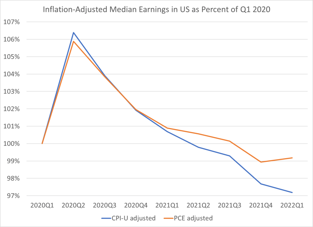
This chart shows average wage growth adjusted with both of these different measures of inflation, expressed as a percent of January 2020 wages. The CPI-U adjusted wages (blue line) have been falling steadily since the beginning of 2021, though the declines have accelerated in 2022. The PCE-adjusted wages (orange line) have also not performed superbly, but at least they are still 2-3% above January 2020. Still, the picture is not rosy: they’ve basically been flat since mid-2020 and have started to drop in early 2022.
Of course, average (mean) numbers can be tricky and sometimes misleading. What if instead we used median wages? Unfortunately, there is no hourly median wage data that is updated every month. The closest data that I usually look at is median weekly earnings, which is available on a quarterly basis. Here’s what that data looks like, expressed as a percent of the first quarter of 2020. I limit the data to full-time workers, since that should give us a roughly comparable number to the hourly data (hours of work may have changed, but using full-time workers should make it roughly constant).
For median weekly earnings, we can see that the picture is even less rosy. Median earnings have been declining consistently since the second quarter of 2020, regardless of which inflation adjustment we use. The decline in the PCE-adjusted measure isn’t quite as steep since early 2021, but both figures are below the pre-pandemic level, and have been for the past two quarters.
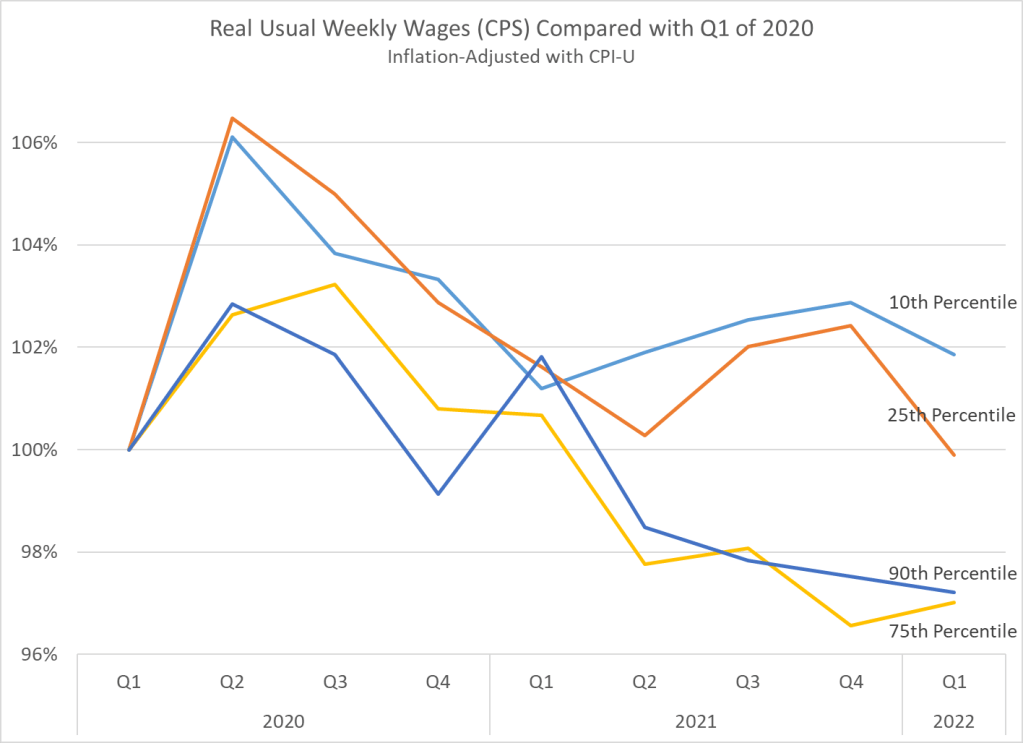
One final note: if we look at weekly earnings across the distribution, and not just at the median, we see something very interesting. Earnings at the bottom of the distribution seem to be performing better than those at the top. In fact, the 10th percentile weekly wage is the only category that is still above pre-pandemic levels. I’m only adjusting using the CPI-U here, but the patterns for the PCE-adjusted earnings would be roughly similar.
We should be cautious about interpreting this data too: if workers dropping out of the labor force are primarily at the bottom of the distribution, it will artificially push up the 10th percentile earnings level. It would be good to know how much of that is going on here. Still, I think this is an important result in the current data.
Now that we’ve all made it through the 2021 tax filing season, it’s worth thinking about a recurring question in tax policy: is it possible that most of us wouldn’t need to go through this annual ritual? Couldn’t the government just tell us how much we owe (or are due as a refund), or better yet, just deduct the correct amount from our paycheck so we’d have paid the right amount?
We need to imagine such a system: it exists in many developed nations around the world! And it’s true that, at least for many taxpayers, the IRS already has all the information on you it needs to calculate your taxes.
But how many US taxpayers would this be beneficial for? A new working paper which tries to quantify this question. In “Automatic Tax Filing: Simulating a Pre-Populated Form 1040,” the authors use a large sample of tax returns to estimate how many taxpayers a pre-filled return would work for. The results are almost split down the middle: it would work well for maybe half of US taxpayers (41-48% of taxpayers, depending on how we are defining successful). For the other half, it wouldn’t give you an accurate estimate of how much tax you owed.
And the errors can be large. For example, the authors report that “two-thirds of the cases where the lower bound approach is inaccurate, the pre-populated liability is higher than the reported liability, with a median gap of $4,200.” Note: looking at the tables, I think they mean to say “mean,” not “median” here, with the median being $1,400. Still, that’s a lot of errors in a direction that would hurt taxpayers if they didn’t fill it out on their own or pay someone to do it. And it’s not just one thing that’s causing pre-filled returns to be wrong. You might think itemized deductions are a big issue, and they are, but only for about 11% of returns (and in only 4% of returns is this the only issue). They find that 9% of returns didn’t even have the reported wages matching what the IRS showed!
Does this mean that pre-filled returns are doomed in the US? Perhaps not! They seem to work much better for younger, single filers, and as well as filers with very low income, as Figure 1 from the paper shows. Even so, the 60-80% success rate (depending on criteria) for very low income taxpayers isn’t especially encouraging. But one upshot of a pre-filled return is that there are possibly millions of taxpayers (maybe 8 or 12 million?) that don’t file a return because they aren’t legally required to (too low income), but they would benefit if they did because of refundable credits like the EITC and Child Tax Credit.
Maybe there is a compromise position. The IRS could send you a “suggested tax return,” but allow you to modify it. I suspect that, in most cases, those who are currently paying for a person or software to do their taxes would still do it. You can’t know if you are in the one-half of taxpayers where this information is accurate! The IRS could provide a list of “common reasons why you may be in the half of pre-filled tax returns that are wrong,” but we’re still shifting the burden back to the taxpayer.
I would like to suggest, instead, that there are a few changes we could make to our tax system (“simplifications,” if you will) that might make pre-filled returns much more viable.
A recent analysis by the Kaiser Family Foundation of CDC data suggests that about 234,000 COVID deaths in the US could have been prevented if everyone was vaccinated. That’s about 25% of all COVID deaths throughout the pandemic, and about 60% of COVID deaths since June 2021 (roughly the time when most older adults in most states had had a chance to be vaccinated).
The first way to think of that death rate is tragic, given that so many lives could have been saved. Rather than being the high-income nation with the highest COVID death rate, the US could have been more in line with countries like Italy, the UK, and France. The US actually had a lower COVID death rate than Italy and the UK when the vaccine roll-out began, and today we could be at about France’s level with better vaccination rates.
But there’s a flipside to the KFF numbers. If 60% of COVID deaths since June 2021 were preventable, that means 40% weren’t preventable. Furthermore, the same data show that about 40% of COVID deaths in January and February 2022 were fully vaccinated or had boosters. That sounds like the vaccines might not work very well! So what does this all mean? Let’s dig into the data from the CDC a little bit.
The first, and most important thing, to recognize is that most American adults are vaccinated (about 78%), so unless vaccines are 100% effective (and they aren’t, despite some public officials overenthusiastic pronouncements early in the vaccine rollout), there are still going to be a lot of COVID deaths among the vaccinated. If 100% of the population was vaccinated, 100% of the deaths would be among the vaccinated. The key question is whether vaccines lower the chance of death.
We’ve talked a lot about vaccines on this blog, including both the benefits of vaccines and how to get people vaccinated. For example, last month I posted about Robert Barro’s estimate on the number of additional vaccines needed to save 1 life. Barro put it at about 250 vaccines. Using some reasonable assumptions, I further suggested that each person vaccinated has a social value of about $20,000. That’s a lot!
But how do we convince people to get vaccinated? Lotteries? Pay them? In addition to just paying them (the economist’s preferred method), another good old capitalist method is advertising (the marketer’s preferred method). And a new working paper tries just that, running pro-vaccine ads on YouTube with a very specific spokesman: Donald Trump.
Running ads on YouTube is pretty cheap. For $100,000, the researchers were able to reach 6 million unique users. And because they randomized who saw the ads across counties, they are able to make a strong claim that any increase in vaccinations was caused by the ads. They argue that this ad campaign led to about 104,000 more people getting vaccinated, or less than $1 per person (the actual budget was $96,000, which is how they get 93 cents per vaccine — other specifications suggest 99 cents or $1.01, but all of their estimates are around a buck).
Considering, again, my rough estimate that each additional vaccinated person is worth $20,000 to society (in terms of lives saved), this is a massive return on investment. Of course, we know that everything runs into diminishing returns at some point (they also targeted areas that lagged in vaccine uptake). Would spending $1,000,000 on YouTube ads featuring Trump lead to 1 million additional people getting vaccinated? Probably not quite. But it might lead to a half million. And a half million more vaccinated people could potentially save 2,000 lives (using Barro’s estimate).
I dare you to find a cheaper way to save 2,000 lives.
Inflation is definitely here. The latest CPI release puts the annual inflation rate in the US at 8.5% over the past 12 months, the highest 12-month period since May 1981. That’s bad, especially because wages for many workers aren’t keeping up with the price increases (and that’s true in other countries too).
But what about other countries? Many countries are experiencing record inflation too. The same day the US announced the latest CPI data, Germany announced that they also had the highest annual inflation since 1981.
Using data from the OECD, we can make some comparisons across countries during the pandemic. I’ll use data through February 2022, which excludes the most recent (very high!) months for places like the US and Germany, but most countries haven’t released March 2022 data quite yet.
Let’s compare inflation rates and GDP growth (in real terms, also from the OECD), using the end of 2019 as a baseline. We’ll compare the US, the other G-7 countries, and several broad groups of countries (OECD, OECD European countries, and the Euro area). The chart below uses “core inflation,” which excludes food and energy (below I will use total inflation — the basic picture doesn’t change much).
Last week President Biden released his Fiscal Year 2023 budget proposal. The annual release of the budget proposal is always exciting for economists that study public finance. The president’s proposal is the first step in the federal budgeting process, which in some cases leads to the full passage of a federal budget by the start of the fiscal year in October (though perhaps surprisingly, the process rarely works as intended).
This year’s budget is especially interesting to look at because it gives us our first look at what post-pandemic federal budgeting might look like. And while the budget has a lot of detail on the administration’s priorities, I like to go right to the bottom line: does the budget balance? What are total spending and revenue levels?
The bottom line in the Biden budget this year is that permanently large deficits are here to stay. Keep in mind that a budget proposal is just a proposal, but it’s reasonable to interpret it as what the president wants to see happen with the budget over the next 10 years (even if Congress might want something different). Over the next 10 years, Biden has proposed that budget deficits remain consistently right around 4.5% of GDP, with no plan to balance the budget in the near future.
How does this compare to past budget proposals? For comparison, I looked at the final budget proposals of Biden plus his two predecessors. I start Obama’s in 2021 to match Trump’s first year, and all three overlap for 2023-2026. I put these as a percent of GDP so we don’t have to worry about inflation adjustments (though we might worry about optimistic GDP forecasts, see below).